Gym-Lattice: RL environment for the protein folding problem
It turns out that my brief soirée with reinforcement learning (RL) became a long dance. I started watching David Silver’s lectures, and seriously considered doing a pet research project in RL. Good thing, deep in my lab’s archives, I found a gem of a problem that may be solvable by reinforcement learning— protein structure prediction. In this post, I will walk you through the first step of my journey in RL-plus-bioinformatics by creating a Gym library for determining protein structures.
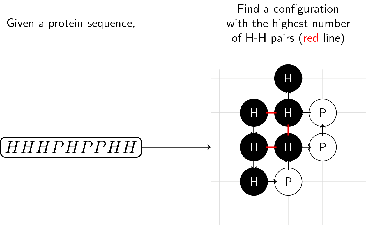
The main idea is that given a protein sequence, we wish to infer what it looks like. However, determining a protein structure in the molecular level is computationally-intensive. Folding@Home is a good example. It implements a distributed computing scheme to use a volunteer’s machine idle time (from PS4 to your web browser) in order to simulate thousands of protein configurations. For our case, we start with simple protein abstractions that are computationally manageable.
- The 2D Hydrophobic-Polar (HP) Lattice Model
- Protein Folding as a Reinforcement Learning (RL) Problem
- The Gym-Lattice Environment
The 2D Hydrophobic-Polar (HP) Lattice Model
The HP Lattice Model is a seminal work that describes proteins in the lens of statistical mechanics (Lau and Dill, 1989). Simply put, it gives us a handle to tackle the protein folding problem in a more tractable fashion. Furthermore, it has been proven that the HP Lattice problem is NP-complete (Berger and Leighton, 1998), joining the ranks of our well-loved travelling salesman and graph coloring problems.
As a result, we can apply optimization techniques such as dynamic programming to solve HP lattices. Because we are doing RL, we will attempt a solution based on markov decision processes (MDPs). First, let’s examine the characteristics of a protein lattice.
Treat it like a game
The goal is simple. Given a protein sequence made up of H and P “molecules,” find the most stable configuration. That is, the config with the highest number of adjacent H molecules (corresponds to the configuration with the lowest energy).

We start with an initial molecule (as per the example above, it’s H), and decide where to put the next molecule: up (U), down (D), left (L), or right (R). We do this until all molecules are placed or if we accidentally trapped ourselves in the sequence.
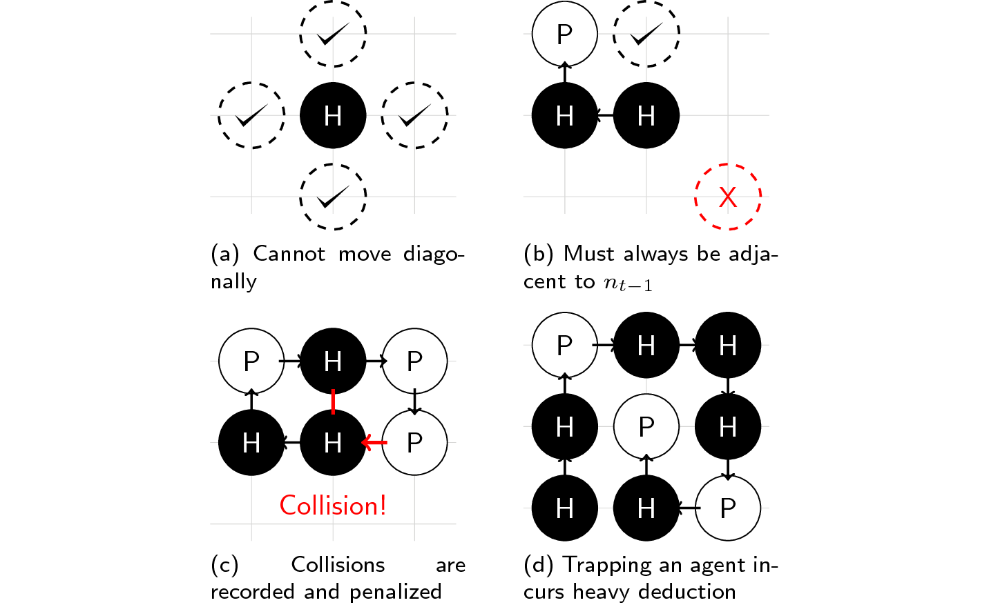
That’s it! However, there are some rules that must be followed while playing this game:
- You cannot move diagonally (only L, R, U, or D).
- You should only put a molecule adjacent to the previous one.
- Placing a molecule on an occupied space is penalized.
- Trapping yourself and failing to finish the task incurs heavy penalty.

As you can see, the HP Lattice model is a very simple abstraction of actual proteins. We only deal with two types of molecules (not 20 amino acids nor \(20^3\) codon combinations), we only work inside a 2-D planar surface, and our objective function (number of H pairs) is a thermodynamic interpretation of how protein molecules behave.
However, solving this problem can help us incrementally solve lower-order abstractions of the protein folding problem, and who knows? Lead us to finally solve how proteins behave in a molecular level.
Protein Folding as an RL Problem
We’ve seen RL being used successfully in games (Mnih, Silver, et al., 2013). Perhaps, formulating protein folding as a sequence of states, actions, and rewards like a game opens up the possibility of solving this via reinforcement learning. First, I will discuss what a typical RL framework looks like, then, we’ll start formulating the protein folding problem as an RL problem.
A typical reinforcement learning problem
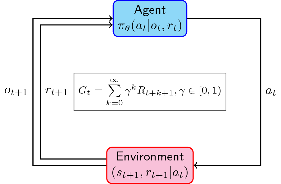
Most reinforcement learning problems are formulated as the following (Sutton and Barto, 1998):
- We have an agent (\(\mathcal{A}\)) that decides an action \(a\) given an observation \(o\) and reward \(r\). Sometimes, the agent’s policy (how it acts given an observation and reward) is parameterized by \(\theta\). It could be a neural network with weights \(\theta\).
- This action goes into the environment (\(\mathcal{E}\)) that takes the agent’s action, determines the equivalent reward \(r\), and updates its state \(s\).
- The next state \(s_{t+1}\) and reward \(r_{t+1}\) is then transferred back to the agent for deciding the next action. Just a note: sometimes we have partially-observed cases where \(s_{t+1} \neq o_{t+1}\). Imagine the fog-of-war in DoTA where you cannot see beyond your visibility range. Ours is fully-observed where \(s_{t+1} = o_{t+1}\) (like chess, you can see the position of all pieces.)
The goal (\(\mathcal{G}\)) then is to maximize the expected reward for all timesteps. For a more thorough discussion of RL, please check Sutton’s book that I referenced below. For a more leisurely yet informative read, check out this great post from Thomas Simonini.

Reinforcement Learning + Protein Folding
Now that we have a rough idea of how reinforcement learning works, we can then combine our knowledge of the protein folding game to create our framework:
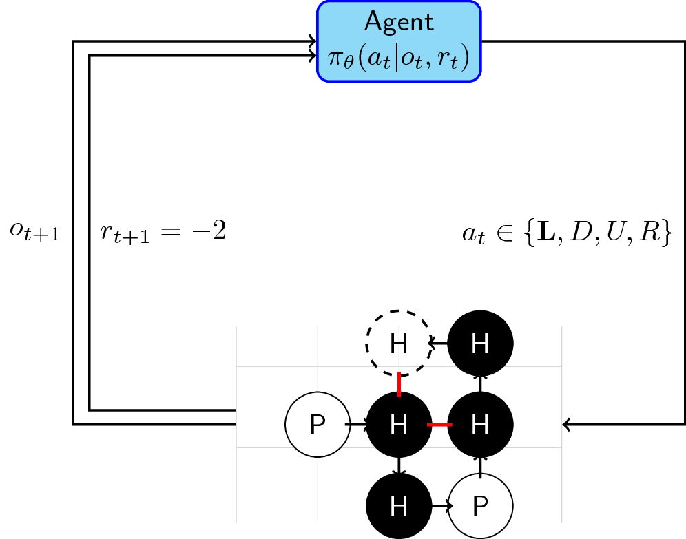
- Our agent (\(\mathcal{A}\)) takes the current state of the lattice plus the reward, and depending on its policy, outputs an action \(a \in \{L,D,U,R\}\) to place the next molecule.
- The environment (\(\mathcal{E}\)) takes this action and updates the lattice by placing the next molecule on the location decided upon by the agent. Afterwards, it computes the number of adjacent H-H pairs that are not consecutive inside the sequence. More formally:
- The agent takes this next state and reward (energy function) and again decides where to put the next molecule until all molecules have been placed. An episode ends when the whole sequence has been exhausted or when the agent was trapped.

For RL practitioners, it is obvious that the sign of the reward is a bit funky. Negative rewards often mean penalties. We wil still modify this reward function as you will see in the gym-lattice environment.
The Gym-Lattice Environment
My project aims to provide an environment (\(\mathcal{E}\)) that simulates
the protein folding problem for training RL agents. It follows a similar API
with OpenAI-Gym, and is built from primitives
found in the Gym library. This means that
the common step(), reset(), and render() methods are available. You can
find the Github link here and
a good Reddit discussion of the project
here.
- In
gym-lattice, the state \(s\) is represented as a 2D-matrix \(S \in \{-1,0,+1\}^{2}\). The observation-space is defined asBox(high=1, low=-1, shape=(2*n+1,2*n+1), dtype=int)+1represents hydrophobic (H) molecules-1represents polar (P) molecules; and0represents unassigned spaces in the grid.
- Your agent can perform four possible actions: 0 (left), 1 (down), 2 (up), and 3 (right). The number choices may seem funky at first but just remember that it maps to the standard vim keybindings.
- An episode ends when all molecules are added to the lattice OR if the sequence of actions traps the polymer chain (no more valid moves because surrounding space is fully-occupied). Whenever a collision is detected, the agent should enter another action.
Small note about the reward function
The reward function \(r\) has been modified. For every timestep, it gives sparse rewards \(r_{t}=0\). The energy function is only computed at the end of the episode (when all molecules are placed). Whenever the agent collides at a specific timestep, a collision penalty is computed. Overall, the reward at t \(r_{t}\) is computed in the following manner:
# Reward at timestep t
reward_t = state_reward + collision_penalty + trap_penalty
- The
state_rewardis the number of adjacent H-H molecules in the final state. In protein folding, the state_reward is synonymous to computing the Gibbs free energy, i.e., thermodynamic assumption of a stable molecule. Its value is 0 in all timesteps and is only computed at the end of the episode. - The
collision_penaltyat timesteptaccounts for collision events whenever the agent chooses to put a molecule at an already-occupied space. Its default value is -2, but this can be adjusted by setting thecollision_penaltyat initialization. - The
trap_penaltyis only computed whenever the agent has no more moves left and is unable to finish the task. The episode ends, thus computing thestate_reward, but subtracts a deduction dependent on the length of the actual sequence.
Basic Usage
It’s very simple to use gym-lattice. Once you have your agent ready, just
call the step(action) function to input your action. Remember that at the
beginning of each episode, you must reset your environment. Below is a basic
skeleton of how to use this package:
from gym_lattice.envs import Lattice2DEnv
from gym import spaces
import numpy as np

np.random.seed(42)

seq = 'HHPHH' # Our input sequence
action_space = spaces.Discrete(4) # Choose among [0, 1, 2 ,3]
env = Lattice2DEnv(seq)

for i_episodes in range(5):
    env.reset()
    while True:
        # Random agent samples from action space
        action = action_space.sample()
        obs, reward, done, info = env.step(action)
        env.render()
        if done:
            print("Episode finished! Reward: {} | Collisions: {} | Actions: {}".format(reward, info['collisions'], info['actions']))
            break
Of course, at each step, you can call render() to see what the lattice looks
like in your console:


Last Notes
I haven’t trained an agent yet to solve this problem, but one idea I have in mind is by using a Deep Q-Network with a convolutional layer to take-in the grid, and is connected to a Fully-Connected Network to output an action. I’ve been very busy with thesis lately so we’ll see what happens in the future.
References
- Lau, Kit Fun and Ken A Dill (1989). “A lattice statistical mechanics model of the conformational and sequence spaces of proteins”. In: Macromolecules 22.10, pp. 3986–3997.
- Berger, Bonnie and Tom Leighton (1998). “Protein folding in the hydrophobic-hydrophilic (HP) model is NP-complete”. In: Journal of Computational Biology 5.1, pp. 27–40.
- Mnih, Volodymyr, Koray Kavukcuoglu, David Silver, Alex Graves, et al. (2013). “Playing atari with deep reinforcement learning”. In: arXiv preprint arXiv:1312.5602.
- Sutton, Richard and Barto, Andrew (1998). Reinforcement Learning: An Introduction Vol. 1 No. 1, Cambridge: MIT Press.
