A brief soirée with reinforcement learning

Update (2018-08): I got an internship offer in Preferred Networks! This year, the intern task is about Adversarial Examples. Awesome task, but I’m not sure if I can share my solutions anymore.

Given the recent success of AlphaGo and OpenAI’s win in DoTA, I decided to dedicate a few weeks studying reinforcement learning (RL). It turns out that RL is a different ball game, and in effect, I need to learn a whole new schema of concepts and ideas. It was overwhelming at first so to just dip my toes in RL, I decided to make a small project.

Good thing, I found this problem set from Preferred Networks. It’s actually a set of tasks for their 2017 internship program, and focuses on an RL problem that I presume is beginner-friendly. Too bad I discovered this quite late, it may have been really nice to apply!

So, the challenge is to balance a cartpole by training a reinforcement learning model so that it outputs an action—i.e., move left or right — in order to maximize the reward. There’s also an additional challenge of using only the Python standard library, so usual matrix dependencies such as numpy are forbidden.

Figure: Cartpole simulation from OpenAI Gym.
We’ll be using a simpler one provided by Preferred Networks

I’ll be talking about my project in the following order:

• I’ll explain what the Cartpole environment looks like
• What kind of model I trained to make the decisions
• The optimization algorithm to find the best model parameters
• Combining the three elements above together
• My software implementation of the RL task
• And some analyses of model behaviour!

The Cartpole Environment

The objective of the task is to balance a pole on top of a cart for a given number of timesteps (500 in the default case). The environment ends when you’ve successfully balanced the pole for all timesteps, or when it falls. After that, the environment resets and another episode is called. Each episode consists of resetting the environment and balancing the cartpole until it drops or the 500th timestep is reached. For the PFN task, success is achieved when the pole is balanced for 95 out of 100 episodes.

Figure: The Cartpole Environment.
Given an action, the environment updates its internal state and outputs a new state.
(For now, we’re only considering fully-observed systems)

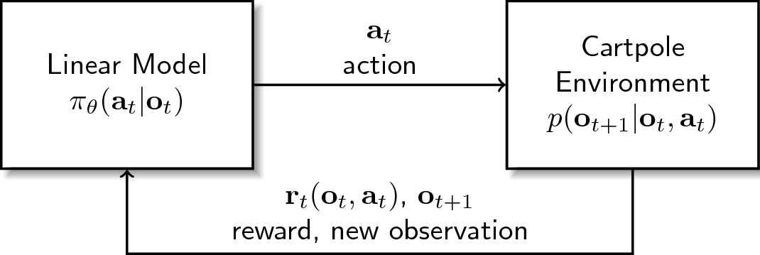
There are various signals that goes in and out the environment:

• \(\mathbf{o}_{t}\), the observation signal going outside that shows the state of the environment at timestep \(t\). There are four observations, \(\mathbf{o}_{t} = \left[o_{1t}, o_{2t}, o_{3t}, o_{4t}\right]\), where each corresponds to a specific aspect of the cartpole: position of cart, velocity of cart, angle of pole, and rotation rate of pole.
• \(\mathbf{a}_{t}\), the action signal going inside that corresponds to the action at a given timestep \(t\). There are only two sets of actions available, \(\mathbf{a}_{t} \in \{-1,1\}\), where \(-1\) is for “move left,” and \(+1\) for “move right.”
• \(\mathbf{r}_{t}\), the reward signal going outside that indicates the reward obtained at timestep \(t\). For cartpole, we receive a \(+1\) reward for every timestep that the pole didn’t fall.

In the software implementation, we have an additional boolean signal done, where done\(\in \{0, 1\}\), that simply indicates if the environment has ended or not. If we designate the Cartpole environment as \(p\), we can obtain a joint conditional probability where the next state is determined by (1) the previous state and (2) the action applied: \(p(\mathbf{o}_{t+1} | \mathbf{o}_{t}, \mathbf{a}_{t})\)

But how do we determine the action \(a_{t}\) to be done? This is where the policy comes in.

Linear Policy

A policy, denoted as \(\pi\), determines the action given the current observation of the environment. In most cases, determining the action is explicitly parametrized. We can then frame the policy in the following distribution: \(\pi_{\theta}(\mathbf{a}_{t} | \mathbf{o}_{t})\). Where \(\theta\) corresponds to the parameters that governs the policy \(\pi\).

Figure: The Linear Model.
The linear model generates an action based on the observation.
In this task, the model is explicitly parameterized

In the case of a linear policy, the action is determined by the sign of the inner product of the observation \(\mathbf{o}_{t}\) and parameters \(\theta\). Simply put,

\[\mathbf{a}_{t} = \begin{cases} +1 & sign(\theta^{T}\mathbf{o}_{t}) > 0 \\ -1 & sign(\theta^{T}\mathbf{o}_{t}) \leq 0 \end{cases}\]

Again, \(+1\) means “move right” and \(-1\) means “move left.” As we can see, the actions are governed by the values of these parameters \(\theta\). At the initial timestep, we can just assign random values to \(\theta\) (in this case we sampled from a normal distribution \(\mathcal{N}(\mu=0,\sigma=1)\)), but we need to find a way to obtain a set of good parameters as we go along, right?

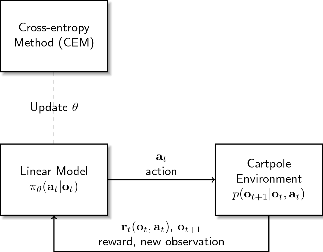
Applying the cross entropy method

In order for our policy to create better decisions, we can employ a scheme to update the parameters every time step. The cross-entropy method (CEM) is an effective way to search for a good set of parameters by updating our current \(\theta\) with the mean of the elite parameters generated from a noisy version of \(\theta\): \(\theta_{i} = \theta + \epsilon_{i}\).

Figure: Cross-entropy Method for updating the parameters.

The algorithm can be seen as follows:

• Until the policy converges, repeat the following:
• Call the current policy parameters \(\theta\)
• For \(i=1,\dots,N\) sample a vector \(\epsilon_{i}\) representing the noise and set \(\theta_{i} = \theta + \epsilon_{i}\)
• For \(i=1,\dots,N\) reset the environment, run the agent for one episode using \(\theta_{i}\) as parameters, and calculate the reward.
• Calculate the mean of the \(\theta_{i}\) vectors whose return was among the top \(100p\%\) and update \(\theta\) to that value.

Here, \(N\) and \(p\) will be our hyperparameters. The former indicates the size of the samples generated from the current parameter, and the latter describes how much of these samples will be taken as elites to obtain the new parameters from.

Combining them all together

Now that we have the environment, the policy, and our optimization algorithm, how can we formalize the problem properly? In addition, we also know that every action results into a new state which results into a different action and so on. In order to represent this concept, we take some inspiration from Markovian decision processes and see that every state-action pairs are related in the following manner:

\[p_{\theta}(\mathbf{o}_{1}, \mathbf{a}_{1}, \dots, \mathbf{o}_{T}, \mathbf{a}_{T}) = p(\mathbf{o}_{1})\prod_{t=1}^{T}\pi_{\theta}(\mathbf{a}_{t}|\mathbf{o}_{t})p(\mathbf{o}_{t+1} | \mathbf{o}_{t}, \mathbf{a}_{t})\]

The left-hand side describes a certain distribution (or if I may, a trajectory) of state-action pairs from the initial time to \(T\). On the right-hand side, we can see that it’s simply a product of all observations and actions occuring at our finit timesteps.

From this, we define the optimization problem as:

\[\theta^{*} = \arg \max_{\theta} \sum_{t=1}^{T} E_{(\mathbf{o}_{t}, \mathbf{a}_{t})~p_{\theta}(\mathbf{o}_{t}, \mathbf{a}_{t})}\left[r(\mathbf{o}_{t}, \mathbf{a}_{t})\right]\]

This means that we need to find the parameters \(\theta^{*}\) that maximizes the expected reward \(r\). Again, the way we achieve this is via the cross-entropy method.

Implementation

Figure: Software Implementation of the RL model

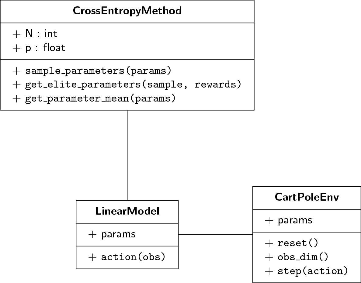
This figure shows how each component of the RL task interacts with one another in terms of object-oriented models. The code repository for this project can be found in this Github link

(CartPoleEnv is based from the PFN’s specifications in the task list, which in turn is loosely-based from OpenAI Gym’s cartpole environment.)

In this set-up, a wrapper class CartPoleEnv interacts with a host program to simulate the cart and pole interaction. The host program, cartpole.out, is provided by PFN, and is written in a C++ file, cartpole.cc. The host program governs the internal logic of the cartpole system (e.g. how \(\mathbf{o}_{t+1}\) is derived from \(\mathbf{o}_{t}\) and \(\mathbf{a}_{t}\), internal physics of the cartpole movement, and the like). To compile the host program, simply execute the following command:

g++ -std=c++11 cartpole.cc -o cartpole.out

The CartPoleEnv class

CartPoleEnv is a wrapper interacting with the host program to provide an API suitable for a reinforcement learning task. It follows a similar API as with OpenAI’s gym. This class consists of the following methods:

• reset() resets the environment into a new initial state \(\mathbf{o}_{1}\).
• obs_dim() returns the number of dimensions in the observation vector (in this case, 4).
• step(action) performs an action, thereby advancing the timestep and updates the internal state of the host program. This returns the new observation, reward (always \(+1\)), and the done boolean signal.

The LinearModel class

LinearModel is a class that takes the observation and performs a relevant action depending on the model parameters. These parameters, theta, are attributes of the object, and is updated every timestep during the optimization process. It only implements a single method:

• action(obs) outputs the action depending on the observation obs and the parameters theta inside the model. This action is either 1 or -1.

The CrossEntropyMethod class

CrossEntropyMethod provides helper functions that fulfills the steps required during the optimization process. It’s not a one-off class unlike the others, but rather an adapter to easily perform various actions:

• init(N,p) takes the hyperparameters N (size of noisy samples generated) and p (amount of elite parameters taken) as its global attributes that will be reused by other methods later on.
• sample_parameters(params) generates a noisy sample of parameters of size N. This returns a matrix of shape (N, len(obs)).
• get_elite_parameters(samples, rewards) takes the noisy samples and their corresponding reward, and retains the top N * p noisy samples with the highest rewards.
• get_parameter_mean(params) takes the elite samples and returns its column-wise mean of shape (len(obs), ).

Given these three components, we can assemble them to create an agent that can be trained in the cartpole task. This is accomplished by the agent.py program found here.

To run the program, simply execute the following command:

./cartpole.out "python3 agent.py"

This runs the agent for 100 episodes with a sampling size of 100 and elite selection of 0.1. Various arguments can be supplied to agent.py to control these hyperparameters:

Arg	Name	Description
-e	episodes	number of episodes to run the agent
-n	sampling size	size of the sample generated by the cross-entropy error
-p	top samples	number of top samples chosen for parameter update
-z	step size	number of steps for each episode
-s	print step	number of steps before printing the output observation
-o	output file	filename to store the win ratio for each episode
-r	random seed	sets the random seed during program execution

To see the list of all arguments, simpy enter the following command:

python3 agent.py -h

When the agent is ran, it will print the observations for every step and the total reward obtained for each episode. In the end, it will show the percentage of episodes that reached a reward of 500. Lastly, running the agent with command-line arguments is demonstrated below:

./cartpole.out "python3 agent.py -e 5 -s 100"

Analysis

For our analysis, we’ll be adjusting three hyperparameters, (1) the amount of noisy samples generated during CEM, \(N\), (2) the number of elite parameters to be taken, \(p\), and (3) the number of steps taken for each episode. We’ll be plotting them against a reward, which I describe as the ratio between the score and the total number of steps. Here, we’ll be examining how each of these hyperparameters contribute to model convergence.

To expound the reward further, take for example our default model with 500 steps per episode. If the RL task was completed successfully, then it has a score of 500, and a reward of 500 / 500 = 1.0. On the other hand, say we only obtained a score of 350 because the pole fell at the 351st timestep. We then compute its reward as 350 / 500 = 0.7. I decided to represent the reward this way to standardize the score once we start changing the number of timesteps.

Adjusting the number of noisy samples

In our model, increasing the number of noisy samples generated during the cross-entropy method has helped hasten convergence. In effect, we can see that a small number of samples (e.g. 25), causes multiple dips during training.

Figure: When the number of noisy samples is increased,
the model converges faster. A low value tends to have several dips during training

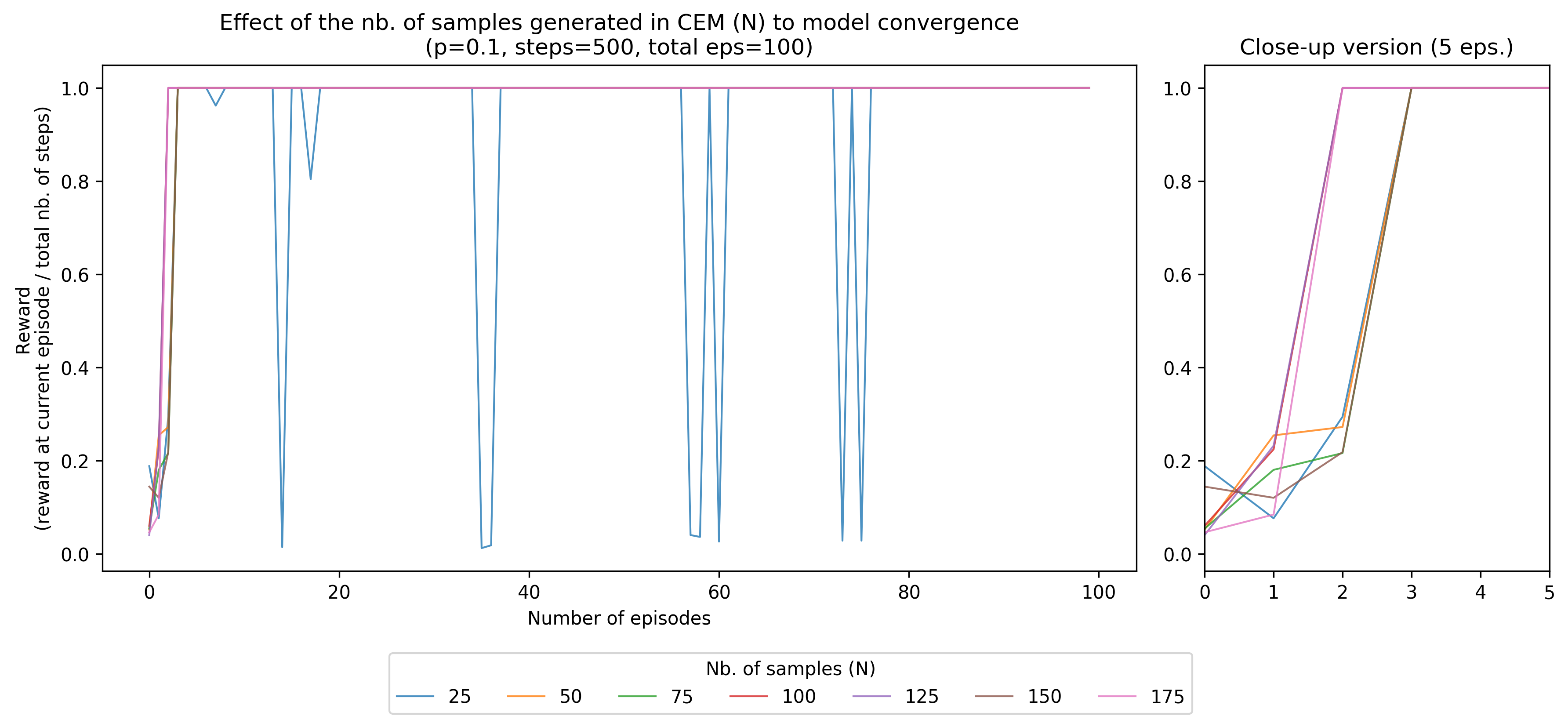
Coming from an evolutionary computation background, I can imagine how \(N\) represents the number of “particles” or “population” of searchers in a search-based method. Increasing the number of \(N\) can help cover all bases in the search-space, whereas decreasing it creates a small cluster that needs to look at the whole space causing the dips.

Adjusting the number of elite parameters

As we decrease the amount of elites, i.e. \(p\) for an elite count of \(N \times p\), the convergence of the model hastens. Interestingly, very high values of \(p\) tend to hurt model convergence as seen in the Figure below:

Figure: When the number of elite samples is decreased,
the model converges faster. Interestingly, higher numbers didn’t converge well

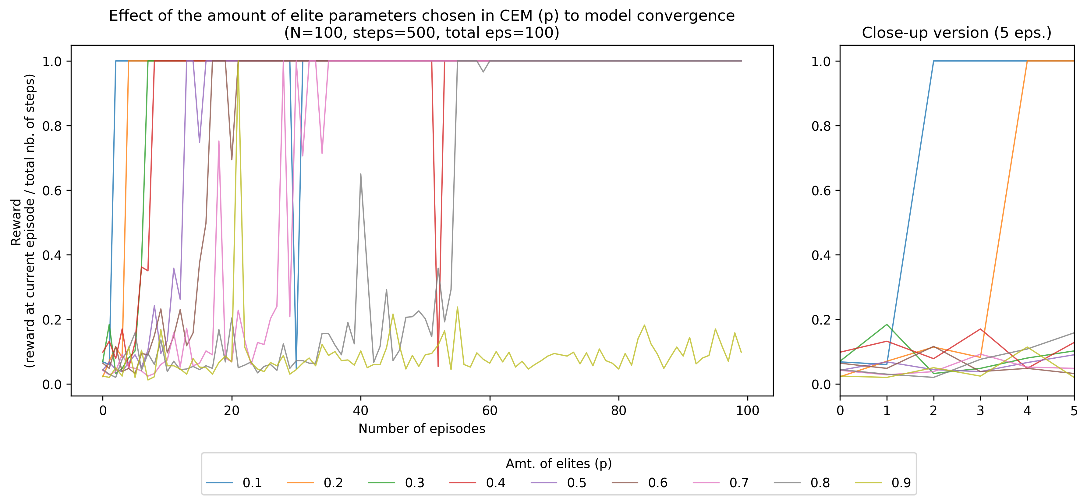
I presume that the number of elites control the exploitation vs. exploration behavior of the model. Decreasing it focuses the distribution of top parameters into its top-performing samples, while increasing it spreads the distribution where all samples contribute to the new parameters.

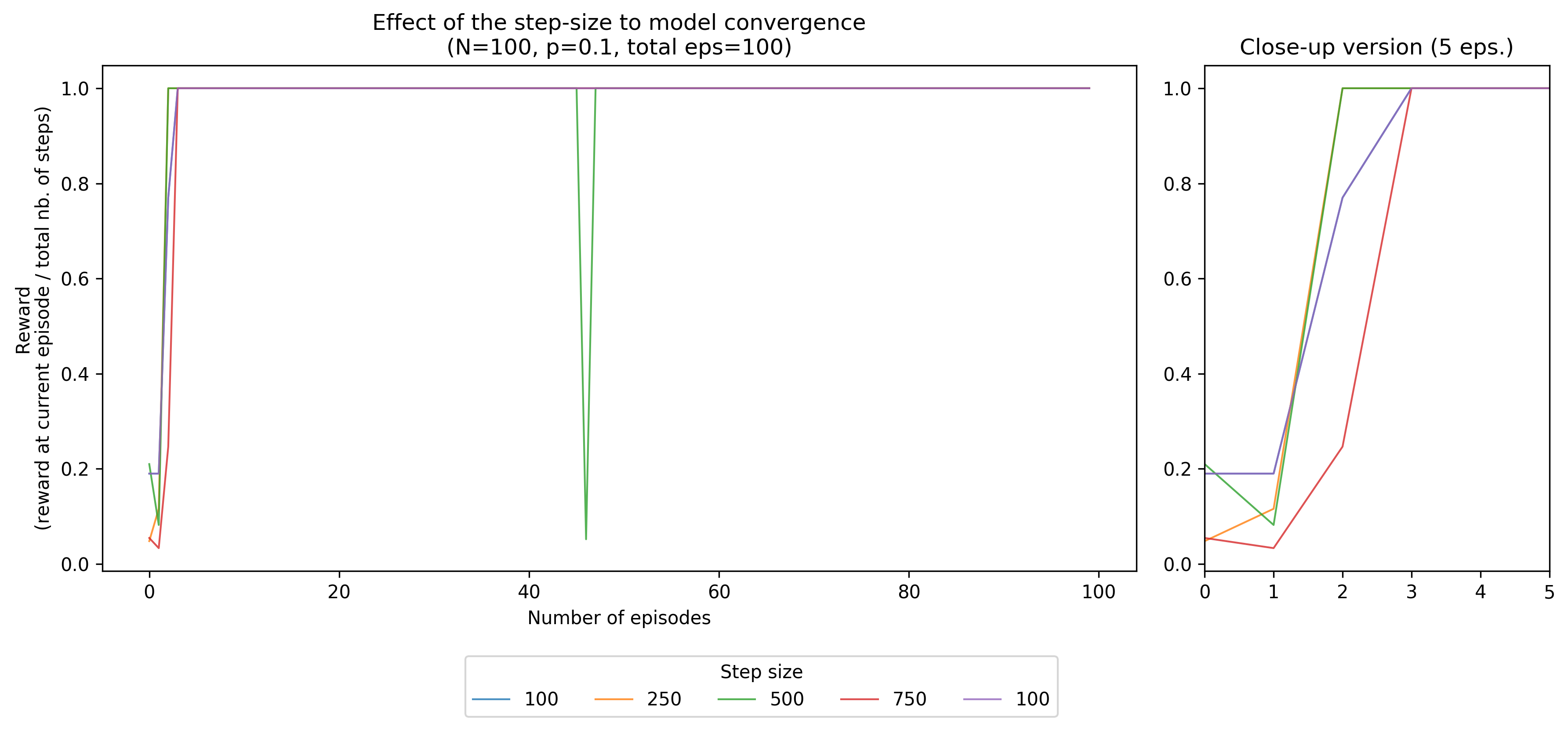
Adjusting the step size

Lastly, we will try to adjust the step size, or the number of timesteps for each episode, and see how it affects the model’s convergence. Interestingly, higher timesteps tend to have a relatively slower convergence, with 750 and 1000 reaching the 1.0 mark later on. Although we had some momentary dip with 500 timesteps, most model variants have a uniform behaviour after convergence.

Figure: Adjusting the model’s number of timesteps

Final thoughts

By doing this project, I realized how rich the literature in reinforcement learning is, and how much problems/problem-variants still remain unsolved. What if we have partial observations? What if there is a delay when passing information? What if there are multiple agents working at once? All of these questions are very interesting to work on in the future!

At the same time, I appreciated how deep learning techniques we have today can be used to model the policy: perhaps a convolutional neural network for an image-like problem, a recurrent neural network for a sequence task and so on. I’m also betting that evolutionary computing methods such as genetic algorithms (GAs) or particle swarm optimization (PSO) can make their resurgence through RL primarily because reward functions need not to be differentiable. Today’s an exciting time for RL indeed! This piqued my interest with RL problems, and I hope I can do research on them in the future!

So here closes my brief soirée with reinforcement learning. I’m aware that there may be some mistakes in my implementation or analysis, so please feel free to message me and point them out!

Changelog

• 10-04-2018: Update figures using Tikz for consistency
• 08-12-2018: Add update on RL task and PFN internship