To preface: the answer to the question of “can we actually build Filipino-centric LLMs?” is definitely YES. The tools are open-source, the recipes are publicly available, and there’s definitely a lot of talent. However, the challenges are two-fold:

1. Building Filipino-centric LLMs does not entail applying Silicon Valley approaches to our local contexts. The capital difference is vast and the ecosystem is different. It’s better to look into how our neighbors (geographically and economically) are doing it, such as Malaysia or Africa.

2. Figuring out real needs is paramount to prevent the project from becoming a vanity training exercise. If the use-case can be solved by the next ChatGPT or Claude release, then maybe it’s not worth going deeper than the application layer.

   Recently, there’s been a lot of talk about retaining ownership over the whole LM development pipeline, hence the proliferation of sovereign LLMs. It’s a common motivation, but I’m not yet well-versed in this topic. The point is: are we building this to fulfill a business need? To include more Philippine languages? To own the LM development stack?

So can we build Filipino-centric LLMs and contribute world-class technologies? My answer is YES, because we Filipinos have the unique qualities and values to do so.

The next step then is to provide an environment where these qualities will flourish. These qualities are: Diskarte, Sipag at Tiyaga, and Bayanihan. Let me explain them in the following sections.

We can build Filipino-centric LLMs and contribute world-class language technologies because we have the unique qualities to do so: Diskarte, Sipag at Tiyaga, and Bayanihan. The challenge then is to create an environment that allows these qualities to flourish.

The slides below are taken from the closing remarks of my talk (about 75% of the talk is about FilBench), but the text doesn’t map to them one-to-one. Just think of this blog post as an extended version of those closing slides.

Diskarte - achieving a goal under extreme constraints

After World War 2, several US Army Willys MB Trucks were left in the Philippines as American troops left the country. There was a shortage of public transportation due to the destruction of infrastructure, and so, we began stripping down these trucks and altering them to add metal roofs, and various paintings and ornaments. This later on became the jeepney or jeep, which is now our cultural icon and the current mode of transportation today.² Diskarte is difficult to translate into English because it can mean many things: resourcefulness, ingenuity, creative thinking, etc. There is this nice paper that talks about this at length, and I encourage anyone to read it. Personally, I see diskarte as the ability to achieve a goal under extreme constraints.

The best way to innovate is similar to how we approached the jeepney: taking these innovations from the Global North and adapting them to our local contexts through ingenuity and resourcefulness.

I argue that the best way to innovate is similar to how we approached the jeepney: taking these innovations from the Global North and adapting them to our local contexts through ingenuity and resourcefulness. Simply importing Silicon Valley approaches is not enough. I wrote about this at length in a recent survey paper, but one approach I’m currently exploring is careful synthetic data generation to address the lack of training data. Synthetic data is now a common approach in training frontier language models, but I believe we can strip it down and, similar to the jeepney, add some ornaments / adjustments to make it work for low-resource languages. I encourage you to read the survey paper, as I mention potential paths for improvement such as creating task-specific small language models, deploying models at the edge, and improving a model’s capabilities through a robust set of harnesses.

That said, the Philippine NLP landscape is constrained in terms of both data and compute. Although there is a significant presence of Filipino speakers and the language is well-represented on the internet, few have transformed this resource into useful, high-quality datasets. This situation is even more pronounced for other Philippine languages. In addition, our compute situation (for both development and deployment) leaves a lot to be desired. We lack the compute infrastructure to train LLMs (Epoch AI Data on GPU Clusters, 2026), and our internet and technology penetration lags behind that of our ASEAN neighbors (ITU Data based on the World Bank).

Sipag at Tiyaga - supporting sustained effort through time

There is a famous saying: “Pag may tiyaga, may nilaga.” Perhaps the nearest English translation I can do is: “If the patience is true, you’ll get a stew.”³ I’d argue that most components of a language modeling recipe (especially in multilingual post-training) are more a test of patience than flashes of insight: collecting enough data through large-scale annotation or synthesis, figuring out the right data mix across many ablations, and ensuring the evals faithfully reflect the capabilities we care about. How, then, can we support these types of activities?

Most components of a language modeling recipe (especially in multilingual post-training) are more a test of patience than flashes of insight.

On the brighter side, I feel quite optimistic about some of the teams scattered across government and academia. For example, E-CAIR has built task-specific systems, and I’ve seen some of their members publishing in *CL and ICML! I also met some folks from AIM last year in Vienna at ACL, so there’s good investment happening there too. And I’ve chatted with a few undergraduate thesis groups in UST and PUP (and I still get the occasional e-mail about calamanCy), so there’s clearly a loose network of groups working on the fringes. What I’m trying to say is that there is talent here willing to do the hard parts—it’s just a matter of getting these efforts more coordinated and aligned.

I’d like to propose two dimensions on how to support these activities: infrastructure and incentives. Infrastructure here can take two forms: compute grants that give people room to experiment, and governance structures with a central decision-maker to keep efforts coordinated. The first one is quite self-explanatory. But I think the second one is much more important.

For example, it is quite difficult to find what is the canonical National AI strategy for the Philippines. The OECD AI Policy Navigator and UNESCO points to NAISR v2 which is from DTI, but the website says it was superseded by another Philippine AI Strategy Roadmap by DOST. Now, the only DOST-related roadmap I can find is this slide deck, but that can’t be it, right?

Bayanihan - collective action to achieve a goal

I always find the imagery of bayanihan inspiring. It’s now uncommon today due to most houses being made of concrete, but the spirit of bayanihan still lives: I remember back in high school when we had Brigada Eskwela and gathered together (my classmates, teachers, and even parents) to clean classrooms, or even the disaster relief packages we assembled for victims of typhoon Yolanda back in college. I’d like to think that this is possible in the context of LLM development.

For such a network to work, it has to be focused on a single objective, much like the imagery of bayanihan where the only goal is to move a house from one place to another.

I wrote about this last year, and I still believe in the capability of grassroots networks. We attempted to build a small research network earlier this year, and while it has been a slow start with a few hiccups along the way, I feel optimistic about what we can achieve next.

However, for such a network to work, it has to be focused on a single objective, much like the imagery of bayanihan where the only goal is to move a house from one place to another. The challenge with loose networks is that everyone has their own priorities and interests, so the effort diffuses. Again, I want to stress that focusing on a single, measurable objective is important. In my opinion, the project should be well-scoped, short-term, and designed so that nodes can pitch in and make drive-by contributions whenever they want. I still have a lot to learn about managing these types of networks, so if you’ve done this before and would like to chat, please reach out!

If grassroots networks are to be multi-sectoral, there has to be a way to align diverse and often conflicting incentives. In academia, for example, there is pressure to secure grants and publications (which, in computer science, means publishing in top conferences and journals). Industry, on the other hand, tends to prefer engineering-heavy, context-specific deployments. As a PhD student, I find that Industry Tracks in conferences are a good avenue for these partnerships: the student gets to work on a concrete project and can even write a paper about it. Finally, the involvement across sectors doesn’t have to be deep on all sides. It could be a donor-recipient setup where, for example, the government provides the problem statement, industry provides the resources, and academia provides the scientific rigor to achieve the goal.

Final thoughts and reflections

If we want to build Filipino-centric language models, we need to build them our way. This entails adapting innovations from other parts of the world to our local contexts and constraints rather than simply importing them (diskarte), creating governance and incentive structures that support long-horizon, experimental work (sipag at tiyaga), and building grassroots networks around a shared, well-scoped goal (bayanihan).

To make this concrete: a good goal would be to train Filipino-centric LMs that cover the country’s major languages (Tagalog, Cebuano, Ilokano, Hiligaynon, Bikol, Kapampangan). The most reasonable approach is to post-train on a strong multilingual base model, then evaluate on a new version of FilBench where all these languages are well-represented. The first major constraint is data, so we need to source it through scraping, native-speaker annotation, or synthetic data generation (diskarte). The second is compute and funding, which calls for partnerships with industry or organizations willing to underwrite them (bayanihan). Finally, much of this work demands sustained experimentation, data ablations, and people willing to see it through (sipag at tiyaga).

As I’ve said, the tools and recipes are publicly available, and I truly believe we have the qualities to make it work. The ball simply needs to get rolling.

This is not a “How to apply to grad school” blog post, but perhaps you’ll find some nuggets of wisdom along the way. If you want an actual guide, I recommend reading John Boaz Lee’s guide (more Filipino context) or Tim Dettmer’s blog post (realistic and quite sobering).

📣 Finally, some news: I started my PhD in Computation, Cognition, and Language at the University of Cambridge this Fall! I also got accepted to universities in the US and Canada, so this admissions cycle was truly a blessing.

All photos you’ll see below were taken by a Gameboy Camera. I realized when writing this blog post that my camera captured all events in the past four years. For more photos, check out my gallery.

The reality of CS grad school applications

Application for PhD programs, especially for machine learning and NLP, has become increasingly competitive. There was a time when I was looking at the newly-admitted PhD students, and it was common to see them with first-author publications in top conferences prior to their PhD. One needs only to look at these tweets from professors and admissions committee members during the Fall 2025 cycle to recognize how competitive the CS PhD applications have been.

Despite my NLP industry experience, I don’t have the academic research backround expected from PhD applicants. Early on, I realized that pivoting from industry to academia would entail a lot of hard work. A part of me thought that maybe I should have just continued to a PhD right after my Masters when the path seemed clearer. But my industry years helped confirm that I genuinely enjoyed research work!

From left to right (–2021): Snippets of my life in Bonifacio Global City (BGC) a few weeks after my time in TM. A bike on display inside Coffee Project, some view of BGC, and a Japanese lantern in The Fort.

I could already imagine the challenges in this transition: relocating to another country, accepting a significant pay cut, and adjusting my life stages (e.g., getting married, starting a family) to align with a new career trajectory. Looking back at 2021, I remember feeling overwhelmed by the self-imposed pressure to make everything fall perfectly into place.

The long road to PhD applications

While working at Explosion, I was fortunate to be exposed to NLP research early on by working on our very first technical report on hash embeddings. This experience gave me the confidence to undertake my own independent work in Tagalog NLP, which led to calamanCy and TLUnified-NER. In addition, doing software engineering work on the Prodigy annotation tool inspired my interest in researching data-centric approaches to NLP.

From left to right (2021—2022): view from my condo when I was working from home in McKinley Hill, the Brandenburg gate during the ExplosionAI meet-up at Berlin, my mechanical keyboard.

My time at Ai2 as a pre-doc was incredibly formative. Working alongside experienced researchers gave me a clearer picture of what academic research entailed and helped me identify the qualities I wanted to develop in myself as I grow into this career. I was also lucky to be part of large collaborative projects like Tülu 3 and OLMo 2 which gave me hands-on experience with frontier model post-training. Working at Ai2 gave me a baseline of what high-quality research looks like.¹ In addition, there’s really something in the air back in the US that made me more ambitious and driven— I hope to bring these qualities wherever I go.

From left to right (2024): the Fremont library where I spent a lot of time writing papers and doing PhD apps, view of the Aurora bridge on the way to the office, the Ai2 logo in the office.

I got lucky because of the people who took chances on me, which is why I developed a mantra over time: people over projects, projects over publications. I prioritize finding people whom I’m excited and energized to work with over specific projects—I believe that every topic is equally interesting given the right people. During the four-year journey, I’ve been fortunate to collaborate with researchers from different places who shared my interests, particularly in multilingual NLP. Everyone I worked with made me feel welcome, and I hope I can be that person for another aspiring researcher in the future.

I’ve developed a mantra over time: people over projects, projects over publications.

From left to right (2024): snippets of my life in Seattle including the Fremont artwork, the pottery studio at Yu Tang Ceramics, and the Farmer’s Market in downtown.

My Masters professor, Jinglu Hu, also supported me all the way during my PhD applications. He was happy to write me a recommendation letter, and I’m more than happy that he wrote it—it felt like things had gone full circle. I have fond memories of Waseda back in 2016, and that time was formative in my career.

On the admissions cycle

The admissions cycle spanned three months, from December to February, with the earliest deadline on December 4. Because I also had to prepare for my wedding in December, I tried to finish all applications and essays by November. I vividly recall arriving at the library as soon as it opened and remaining there until it closed. The holiday season also brought a reflective mood, with fewer people around and a quieter atmosphere, I was able to reflect on what type of research I wanted to pursue.

From left to right (2024-2025): snapshots during the admissions season: writing essays in the Fremont library or in Cafe Ladro, buying food from PCC.

I applied to 7 programs, and they’re actually quite expensive! I missed some of the fee waiver deadlines because I was busy, so I had to shell out $1,350 to $1,500 for application fees. In addition, some universities require official TOEFL scores, so you also have to pay TOEFL fees in order to send your test results to those universities (~$35). Don’t make my mistake and keep in mind that fee waivers exist and most universities are generous, especially for international students, but just note that grad school apps can be very expensive.

From left to right (2024-2025): The PhD applications forced me to think whether I want to stay in the US or move again abroad. Some snippets of my life (from left to right): a bike in Roosevelt Island, my apartment at Phinney, a US flag in Grand Central Station.

By January, I started receiving interview invites. I had a mix of interview formats during this cycle: a research presentation, a short 15-20 minute informal chat, and a formal interview. The last two weeks of January and the early weeks of February were the most intense, as they involved a lot of waiting and uncertainty. I tried to keep myself busy, focusing on work and my current research projects— those were the longest two months I had ever experienced.

On choosing PhD programs

One of the hardest challenges in entering a PhD is balancing your career aspirations and future life plans. This is especially true for someone like me in their early 30s: a PhD program can take 4-6 years, pays lower than your typical software engineering job, and will coincide with the time when I might want to start a family. Making this decision in my thirties is different from if I had made this decision during my twenties. Getting into a PhD becomes a life decision more so than a career decision.

From left to right (early 2022 and 2023): coffee shop where my wife and I talked about our plans, my room during a Holy Week retreat in Sacred Heart, our engagement ring.

I’d like to think that my industry years have matured me well enough to de-risk entering a PhD program. This factored into my choices: will I enjoy my research topic? will I be inspired by my environment? how old will I be after the PhD program and what life/career options will I have by then?

A lot has been written on how to choose PhD programs. My favorite was Tim Dettmer’s post. Based on his blog, I think I went with the Stability perspective. During ACL, I met several folks from Cambridge (although from different departments), and they seem genuinely happy. Interestingly, during the conference, I met an old friend of mine from spaCy and just realized that he was also from Cambridge! In addition, UK is one of the few countries where my wife can stay with me and work. PhD years are long and gritty, and having a rock to lean on is important.

Getting into a PhD becomes a life decision more so than a career decision.

Photos during my PhD visit days in NYC.

Although choosing a PhD program seems like a cerebral choice that entails a lot of calculus, a large part of my decision-making involved a lot of discernment. Attuning myself to my desires and praying over them helped a lot. One thing I’ve learned during this time is that I can never make this decision with absolute certainty. There’s definitely this fear of closing other doors and potential futures—what if you made the wrong choice? Doubt will always be present, and I should welcome that.

Final thoughts

It’s almost November, and my wife and I have been here at Cambridge for almost a month. There’s a lot to say about Cambridge—the collegiate system,² the traditions, the culture, and more. Things still look unfamiliar, but I’m taking my time to let the place reveal itself to me, knowing that we’ll be here for a while. It’s also encouraging to see that Cambridge has a strong support for mature students like me. I’ve met PhDs who also started at the same age as I did, some have even brought their kids! It’s very different from my previous campus tour experience, where most incoming PhDs were fresh from undergrad. In some way, I don’t feel alone and different, and that’s important.

From left to right: Churchill College (a modern college in Cambridge with brutalist architecture), the University Library, a phonebooth repurposed into a library book deposit.

I’m happy to close this chapter that lasted for four years. I’m thankful to all the people who helped me along the way, as I’ve learned a lot about myself and who I wanted to be. The path was long and winding, but I’m happy we made it. The next few years will be equally exciting, but I just want to linger in this moment—that in-between space as you turn the page to another chapter.

Now that I’m past the hump of PhD applications, I’d like to give back: if you’re interested in doing research on Tagalog and Filipino NLP with the intention to publish, feel free to reach out, and I’m happy to mentor you! I can also review research statements, but I’m not an expert!

If you’ve reached this part, dear reader, thank you for reading. Here I am in my matriculation gown!

At the end of 2024, I wrote about my desiderata for Filipino NLP. One of which was evaluation. I said that most of “how we measure LLM capabilities in Filipino are anecdotal: we post a screenshot of ChatGPT writing in Filipino and claim that it already has that capability—we need a systematic approach to evaluating these models.” Fast forward to today, I’m happy that we are now inching towards systematic evaluations for Filipino.

Without further ado, I introduce FilBench, an LLM Evaluation Suite for Filipino!

• Paper: https://arxiv.org/abs/2508.03523
• Code: github.com/filbench/filbench-eval
• Leaderboard: hf.co/spaces/UD-Filipino/filbench-leaderboard

What is FilBench?

FilBench is a (1) benchmark to test LLM capabilities on Filipino, and a (2) leaderboard to track the progress of LLM development for Philippine languages. When building FilBench, I imagine two types of audiences:

• The multilingual NLP research scientist who wants to test whether their new language model generalizes to other languages. FilBench aims to provide a robust and comprehensive evaluation suite for Filipino tasks and use-cases.

• The language model developer who wants to know which language model fits best for the application their building. The FilBench leaderboard provides a detailed breakdown of a model’s capabilities, and analyses of the parameter- and cost-efficiency of such models.

When building FilBench, we took stock of what the Philippine NLP research community are evaluating pre-ChatGPT language models upon. Although they are good at understanding language system capabilities, they are ill-posed for current LLM evaluation. We then curated these datasets into four main categories: Cultural Knowledge, Classical NLP, Reading Comprehension, and Generation.

Finally, FilBench has been accepted to EMNLP Main! EMNLP is one of the top NLP conferences in the field and getting a paper published in this venue can be competitive. We’re happy with the outcome, so catch Ely and Joseph as they present FilBench in Suzhou, China this November!

On Building FilBench

One thing that I found exciting when building FilBench is that it felt like I’m assembling the Avengers of Filipino NLP. It started with just the three of us— Ely, Conner, and I— working on the Data Is Better Together annotation project from HuggingFace. I’ve met them separately through other projects like SEACrowd and earlier correspondences. Then, we’ve onboarded Joseph and Blaise, who have been working on Filipino NLP since I entered the field. We’re just five right now, but hopefully next time there’ll be more of us.

I find grassroots projects like this to be appealing, given that all of us are volunteers spending our free time on FilBench. We automatically pass the “will-they-care-about-this-project” bar, making collaboration smoother. There were hurdles too, such as scrounging up compute for running evals, or finding the right time across five timezones. But the scrappiness of the group is energizing, and it allowed us to iterate and build FilBench despite little to no resources.

In addition, it was also nice working with the OpenEvals team at HuggingFace, since they help maintain lighteval, the evaluation framework we used for Filbench. I’m also thankful to Nathan Habib, Clementine Fourrier, and Daniel van Strien for their feedback on the official HuggingFace blog post. Furthermore, FilBench is now part of the official community evaluations on lighteval, so check it out there!

We have some interesting projects lined up and there’s definitely still some space on the bench. I’m very optimistic about the future of Filipino NLP research, and would love to broaden my collaborations more. So if you’re interested in collaborating with us, then reach out!

My next plans for Filipino NLP

For me, the next few months will bring about a lot of change and adjustment. I’m currently vacationing in the Philippines until October so I’m yet to initiate new research projects for the latter half of the year. However, I haven’t been idle: I’ve been shaping up ideas and talking to some people so hopefully I’m back in action by Q4.

• On FilBench v2: I have a lot of new ideas for FilBench v2. However, I want to maintain my key priority for developing FilBench, i.e., to improve the scope of Philippine languages in our benchmark. More specifically, my metric of success for FilBench is to cover all major regional languages in the Philippines.

  We also have some plans regarding a cost-efficient and mini version of FilBench. This allows model evaluators to easily get feedback on their FilBench scores without running the full set. The details are being finalized, but the goal is to release FilBench-Mini by the end of the year.

• On Filipino NLP: Most of what I’ve mentioned in my desiderata still hold. Now that I’m heading towards my PhD, I’m also figuring out how I can balance my interests in Filipino NLP and my general PhD research project. Nevertheless, I believe our efforts on FilBench have proven that grassroots and volunteer-led research projects can be successful.

I’d like to collaborate with organizations who can provide compute. I have some ideas on low-resource LLM training and data curation (with Filipino as a case study). Training a Filipino-centric LLM is often a conversation topic I hear a lot, but I think there should be some finesse on executing and framing this project, so that it becomes impactful and not “yet another” LLM that the next frontier LLM like GPT-4.1 can easily beat.

Final thoughts

Overall, I’m very happy with the progress we had in FilBench. It is a good project where I was able to collaborate with other contemporaries in Filipino NLP, and resulted in a main conference acceptance. Projects like these don’t stop after publication— in fact the whole “Filipino NLP” project is just beginning. With FilBench, we now have a comprehensive and easy-to-run benchmark for LLMs. The next step is to then figure out what kind of model—or more specifically, what type of pre/post-training data, architecture, training paradigm— can top this leaderboard.

If you’re interested to work on language-specific evals and Filipino NLP in general, just shoot me an e-mail and let’s chat!

Citation

@article{miranda2025filbench,
  title   = "Fil{B}ench: {C}an {LLM}s {U}nderstand and {G}enerate {F}ilipino?",
  author  = "Miranda, Lester James Validad and 
            Aco, Elyanah and 
            Manuel, Conner and 
            Cruz, Jan Christian Blaise and 
            Imperial, Joseph Marvin",
  journal = "arXiv preprint arXiv:2508.03523",
  year    = 2025
}

Works I presented during the conference

Self-promotion: I had four papers accepted in the ACL Main Proceedings, three of which I was the first or co-first author on (all in the Resources & Evaluation track):

• Hybrid Preferences: Learning to Route Instances for Human vs. AI Feedback
  TLDR: We find that some preference instances are better annotated by humans than by language models (LMs). We use that information to train a hybrid preference router (HyPER) that allocates instances to either humans or LMs.
• M-RewardBench: Evaluating Reward Models in Multilingual Settings.
  TLDR: We introduce a new benchmark for evaluating reward models (RMs) in 23 diverse languages. By evaluating several RMs on M-RewardBench, we uncovered signficant gaps in RM performance between English and non-English languages.
• The UD-NewsCrawl Treebank: Reflections and Challenges from a Large-scale Tagalog Syntactic Annotation Project
  TLDR: We introduce the largest Tagalog treebank to date, 100x larger than previous treebanks. By building this treebank, we stretch the limits of the Universal Dependencies framework and challenge its “universality.”

And a big collab project from SEACrowd:

• Crowdsource, Crawl, or Generate? Creating SEA-VL, a Multicultural Vision-Language Dataset for Southeast Asia
  TLDR: We present SEA-VL, one of the largest open-source initiatives to develop high-quality and culturally-relevant data for SEA languages. We also highlight representation gaps in SEA, especially for vision-language models.

Really, four papers?! This seems like a big feat, but these works were completed at different times—it’s just that the timing led them to be published simultaneously. In fact, HyPER was a reject from ICLR that we further refined, and my involvement in UD-NewsCrawl started way back in 2023. Good research takes time, and I’m lucky to have great collaborators during these long periods of work.

Papers that piqued my attention

I enjoyed going through the poster presentations during the conference. Since I was presenting, I wasn’t able to attend most of the Main posters. However, I had a great time talking to other researchers in the other sessions!

• Language Models Resist Alignment: Evidence from Data Compression: It’s one of the best papers of ACL and presents a physics-inspired view of post-training behaviour. According to the paper, post-trained LMs exhibit some kind of elasticity, where it reverts back to its behaviour distribution during pretraining when finetuned further. The rest of the work is an analysis of this elasticity, where they found that it positively correlates with increased model size and expansion of pre-training data.

• Building Better: Avoiding Pitfalls in Developing Language Resources when Data is Scarce: A good paper that examines the patterns in language resource development form a survey of several NLP practitioners. It also highlights some potential systemic issues with large-scale community efforts such as credit attribution. I find this paper thought-provoking as it looks into the meta of language resource development and reveals issues that we tend to take for granted.

• Can External Validation Tools Improve Annotation Quality for LLM-as-a-Judge?: This is an interesting paper that examines how tools can improve annotation quality in LLM-as-a-judge scenarios. I’ve been working in finetuning LMs for tool-use at Ai2, and I’m very curious of its applications in some of the domains I care about. There is good empirical evidence for using tools during annotation, and I’m excited to see where else we can apply this framework.

Honorable mentions:

• A Perspective on LLM Data Generation with Few-shot Examples: from Intent to Kubernetes Manifest: fun industry-track paper that solves the problem of writing annoying Kubernetes configs! Tickled the software engineer in me.
• PLAY2PROMPT: Zero-shot Tool Instruction Optimization for LLM Agents via Tool Play: an interesting framework for refining tool instructions. Might be useful for improving the quality of synthetic tool-use data.
• Automatic Transmission for LLM Tiers: Optimizing Cost and Accuracy in Large Language Models: a good addition to the literature of LLM routing. Can even be useful for some LLM-as-a-judge applications.

Miscellaneous

• I attended the SEACrowd Birds-of-a-Feather (BoF) session! Finally, I’ve met my long-time collaborators. I’ve been involved with the SEACrowd group during their initial project, so it’s nice to meet Holy, Samuel, and Aji in person. During the BoF, we talked about what is “enough” for Southeast Asian NLP, what’s missing (it’s always money), and what are our current successes. I honestly look forward to SEACrowd events. I traveled to ACL alone, so being with some familiar faces gave me a feeling of having a home base in a sea of strangers.

• Met with some Pinoy NLP researchers. I’m also glad to see Filipinos publishing in these top NLP conferences. I met with some folks from the Asian Institute of Management (Sir Chris, Japer, K-Ann), SEACrowd (Blaise and Anton), AI Singapore (Railey), and Radboud University (Jane). Data science in the Philippines is a small world: each of us were connected in one way or another (either we’re from the same high school, college, job, etc.). I was very happy to see Pinoys and almost shouted Uy pilipins! upon meeting them.

• Thank you for the water, kind stranger! During the second day of the conference, I was presenting two posters at the same time! It was quite intense as I jump from one work to another. Add Vienna’s summer heat and I was definitely sweaty and haggard. Suddenly, a kind stranger offered me some water and I felt refreshed and energized. It was a nice gesture and now a core memory of my conference experience. I wasn’t able to catch their name, but if you’re reading this: thank you for the water, kind stranger!

Final thoughts

Attending ACL 2025 is a great way to close my pre-PhD years and start my new journey as a PhD student. As my first NLP conference, ACL gave me a favorable first impression of the community at large. Perhaps I’ve been lucky with the people I’ve talked to, but everyone was warm, friendly, and welcoming. Good vibes all throughout, no notes.

Also, I enjoyed writing this field report: it’s a good exercise for me to synthesize things I’ve learned during the conference, and hopefully it’s informative for non-attendees to get an inside look into these academic research events. I admit I haven’t been writing in this blog recently (although in general, I’ve written way more during the past two years), so this might be another way to fill-in those spaces during the year. Hoping to write more field reports in the future! And finally, some photos of my post-conference trip:

In this blog post, I tested LLMs with tool-calling capabilities on the following tasks:

• Task 1: Draw a swordsman: an easy task that generates a static image.

Draw me a pixel art of a swordsman.

• Task 2: Draw a swordsman performing a slashing sequence: a harder task.

Draw a 4-frame spritesheet showing a swordsman performing a sword slash attack sequence, with each frame capturing a different stage of the slashing motion from windup to follow-through.

The characters in Task 1 and Task 2 don’t have to be the same. Task 2 is particularly interesting because creating sprite sheets is a common use-case in game development. It’s also challenging for LLMs since it requires sequential understanding: each frame must logically follow the previous one to create believable animation. Unlike generating a single image, sprite sheets demand consistency in character design, progression, and timing.

Here’s a human baseline from a game I made a few years ago:

Task 1: Swordsman	Task 2: Draw a 4-frame spritesheet of a sword slash attack

I evaluated each LLM’s output using two criteria, each scored from 0 to 3:

• Correctness: Did the LLM follow the instructions accurately?
• Creativity: How original or artistic was the LLM’s approach?

To get a single representative score, I compute the average of correctness and creativity for each task, then average those two task scores together—a benchmark I’ll now dub as SwordsBench score!

You can find the full code on GitHub

Setting up the Agent-Environment Interaction

This project also helped me understand the development workflow for MCPs and LLM agents. I like framing this setup similar to reinforcement learning: we instruct an Agent (an LLM) to interact with the Environment (standardized via MCP) to accomplish a task, as shown in the diagram below:

In the tool-calling paradigm, we instruct an Agent to interact with the Environment in order to accomplish a task. The Agent can be implemented via the OpenAI Agents SDK or natively in Claude Desktop, while the Environment is an MCP server that calls Aseprite commands.

MCP Server Environment

The Environment receives commands from the Agent, executes them, and provides feedback that the agent can use for its next action. Recently, Anthropic released the Model Context Protocol (MCP), which provides a common interface for how agents can interact with any given environment. I think of MCP as a standardized set of affordances for the Agent.

For this project, I used the Aseprite MCP implementation from divii/aseprite-mcp with some slight modifications and bug fixes. The Aseprite MCP server exposes the following tools:

Under the hood, these tools are Lua commands that are sent to the aseprite executable. For example, the draw_pixels tool call is simply a series of img:putPixel commands for drawing pixels:

@mcp.tool()
async def draw_pixels(filename: Path, pixels: list[dict[str, Any]]) -> str:
    ...
    for pixel in pixels:
      x, y = pixel.get("x", 0), pixel.get("y", 0)
      color = pixel.get("color", "#000000")
      # Convert hex to RGB
      color = color.lstrip("#")
      r, g, b = int(color[0:2], 16), int(color[2:4], 16), int(color[4:6], 16)

      script += f"""
      img:putPixel({x}, {y}, Color({r}, {g}, {b}, 255))
      """

    # Submit the script to Aseprite
    execute_lua_command(script)
    ...

Then, the function execute_lua_command calls the aseprite executable and passes the Lua script to the --script argument. You can find the full implementation of the Aseprite MCP server in this repository.

Large Language Model Agent

The Agent has access to tools that interact with the execution environment to accomplish a task. We use language models like GPT-4.1 or Claude Sonnet 4—some of which were trained for tool-use—as agents. Models with tool-use capabilities can output function calls based on the tools in their system prompt. These function calls are parsed by an intermediary layer (such as an MCP server) and passed to the execution environment.

I used the OpenAI Agents SDK to build the Aseprite agent. The implementation is quite straightforward: I just need to create an instance of an Agent class and let it interact with the execution environment (mcp_servers=[server]). For open-weight models, I host them as an OpenAI-compatible vLLM server and pass the server URL to a LiteLLM proxy when instantiating the Agent class.

async with mcp_server as server:
    with trace(workflow_name=workflow_name):
      model = get_model(model_name)
      agent = Agent(
          name="Assistant",
          instructions=system_prompt,
          model=model,
          mcp_servers=[server],
      )

      result = await Runner.run(
        starting_agent=agent, 
        input=request,
      )

When an Agent is instantiated, it contains information about the model it’s using, its system_prompt, and the mcp_servers it’s connected to. I experimented with different system prompts—the one below gave me the best results:

You are a creative and artistic function-calling agent that can use pixel art tools to perform a drawing task. You have a good knowledge of color, form, and movement. Your output must always be saved as an image file in the PNG format. If you encounter an error, find a way to resolve it using other available tools.

To initiate an interaction between the Agent and the MCP server, we simply pass the agent to a Runner class with our actual request as input.

Results

Below are the results of several models on the simple swordsman and spritesheet tasks. The figures below show the best of three agent-environment interactions, selected based on correctness and creativity criteria.

Qwen 3 32B (SwordsBench: 0.25)

Task 1: Swordsman	Task 2: Draw a 4-frame spritesheet of a sword slash attack

Qwen3 performed poorly on both tasks. I can see the attempt to draw a swordsman in Task 1: the brown circle is the head, the cyan rectangle is the body, and the grey rectangle is the sword. However, the Task 2 drawing is poor and doesn’t produce anything recognizable. I actually ran Qwen 3 with both reasoning turned on and off. Generally, using tools with reasoning resulted in better-looking figures, though it took much longer to complete.

Funny enough, when I read the reasoning trajectories, it seems that Qwen 3 likes blaming the tools. It will say something akin to: “the draw_line tool doesn’t work, so I have no way to perform this task” (it actually works). I’m sorry Qwen, but this is a skill issue (minus points for the attitude too).

Task 1 - Creativity (0/3), Correctness (1/3)
Task 2 - Creativity (0/3), Correctness (0/3)

GPT-4o (SwordsBench: 0.75)

Task 1: Swordsman	Task 2: Draw a 4-frame spritesheet of a sword slash attack

GPT-4o’s intent is clearer than Qwen3’s output. The Task 1 drawing can definitely be a swordsman if I squint hard enough. There’s a recognizable sword shape, but the body is either missing or unclear. The Task 2 spritesheet shows promise: there’s clear movement from one sprite to another, and the blue “swordsman” maintains consistency across frames. However, it seems like GPT-4o has taken a lot of creative liberties in designing the swordsman, as the blue blob is hard to identify by itself. This is a good and earnest try.

Task 1 - Creativity (1/3), Correctness (1/3)
Task 2 - Creativity (0/3), Correctness (1/3)

GPT-4.1 (SwordsBench: 1.25)

Task 1: Swordsman	Task 2: Draw a 4-frame spritesheet of a sword slash attack

GPT-4.1 shows a marked improvement over GPT-4o. The Task 1 swordsman is much more recognizable—there’s a clear humanoid figure with distinct head, body, and limbs, but no well-defined sword. The proportions are reasonable and it actually looks like a character you might find in a classic pixel art game. For Task 2, while the character design remains consistent across frames, the animation sequence doesn’t quite work. The “sword” ends up looking more like a gun being held horizontally, and there’s no clear slashing motion or arc. It’s a decent attempt at maintaining character consistency, but fails to capture the essence of a sword attack.

Task 1 - Creativity (2/3), Correctness (1/3)
Task 2 - Creativity (1/3), Correctness (1/3)

Claude Sonnet 4 (SwordsBench: 2.0)

Task 1: Swordsman	Task 2: Draw a 4-frame spritesheet of a sword slash attack

Claude Sonnet 4 is getting there but isn’t quite the most polished. The Task 1 swordsman does look like a proper pixel art character—you can make out the basic humanoid form and it has that classic retro game aesthetic. It’s recognizable as a swordsman even if the details aren’t super crisp.

Task 2 is where things get weird: while there’s definitely a slash motion happening across the frames, the character completely loses all sense of body proportions. The figure becomes distorted and inconsistent, though you can still trace the sword movement from windup to strike. It’s like the model understood the motion but forgot about maintaining the character’s form.

Task 1 - Creativity (2/3), Correctness (3/3)
Task 2 - Creativity (1/3), Correctness (2/3)

Claude Opus 4 (SwordsBench: 2.5)

Task 1: Swordsman	Task 2: Draw a 4-frame spritesheet of a sword slash attack

Claude Opus 4 produces solid results across both tasks. The Task 1 swordsman shows good creativity with a distinctive character design—clear head, body, and sword, though the sword shape could be more refined. What’s particularly interesting is that Opus seems to have developed a consistent character concept: even across different prompts, it drew essentially the same swordsman design.

Task 2 delivers a proper slash sequence where you can follow the sword’s motion from windup to strike, and the character maintains its form throughout the animation. It’s a competent spritesheet that demonstrates understanding of both animation principles and character consistency.

Task 1 - Creativity (3/3), Correctness (2/3)
Task 2 - Creativity (2/3), Correctness (3/3)

Discussion

Recently, I’ve been conducting research on endowing models with tool-use capabilities. I’ve been deep in the modeling side, so it’s interesting to see and address some knowledge gaps from a developer’s perspective. Here are some of my learnings:

Models are constrained by the tools available to them

“Give me a lever long enough and a fulcrum on which to place it, and I shall move the world.”

The Aseprite MCP server exposes basic primitives—from drawing a single pixel to basic shapes. In reality, pixel artists use many other Aseprite features: color pickers, multiple onion frames for animations, and more. This might explain why the resulting artworks look blocky and basic compared to human-created art.

From a developer’s perspective, choosing which tools to expose and their granularity (e.g., drawing pixels → drawing shapes) is crucial for MCP server design. Most models work within the constraints of provided tools, so determining which tools to build gives you the right leverage from a “very-smart-assistant.” From a researcher’s perspective, it would be interesting to endow models with the capability to create their own tools or assess tool quality. I’ve seen this in Claude Code, where it writes Python scripts to perform complex tasks. There are many long-horizon tasks that make this area exciting!

Not all tasks or use-cases require a tool-calling LLM

When I started this project, I was excited about having a language model interact with a program I’ve been using. Now I realize that drawing pixel art might not be the best use-case for a tool-calling LLM. Creating an MCP server requires significant time investment—I could have just drawn inspiration from an image generation model or Pinterest and created the swordsman myself. Better Aseprite MCP use-cases might include asking an AI assistant to export drawings into Godot-compatible spritesheets, recolor artwork with different palettes, or correct pixel dimensions for isometric art. There are many possibilities for augmenting human workflows with tool-use LLMs.

From a researcher’s perspective, it’s worth assessing whether domains and use-cases in famous benchmarks like BFCL truly reflect how tool-calling LLMs are used. Many of these were scraped from GitHub or API repositories, but these APIs’ affordances differ greatly from actual tool usage. For example, the draw_pixel function from my MCP server might be a valid test case, but it doesn’t reflect the complexity and sequential nature of real tool-calling tasks. Perhaps this explains why Claude Code has worked so well and gained traction in the developer community. Instead of going broad, it went deep into a particular use-case—software development—and optimized for that.¹

Final thoughts

In this blog post, I learned about developer tooling for agents by having function-calling LLMs interact with Aseprite. The results were mixed: Claude Opus 4 generated the most creative pixel art while following instructions. I was surprised that models like GPT-4 weren’t very creative. This exercise revealed interesting avenues for future work. I’m curious about endowing LLMs with the capability to create their own tools when necessary. I’m also interested in evaluation, especially for complex and domain-specific tasks. Finally, I’m starting to understand why MCP—or a general protocol for LLM interaction—is important. Writing an MCP server feels more convenient than building REST endpoints. It’s still early, but I hope MCP becomes more prevalent in the future.

The pace of progress in multilingual LLMs has also been relentless this year. We’ve seen several high-profile releases such as Meta’s Llama 3.1, Cohere for AI’s Aya Expanse, and Southeast Asian models such as AI Singapore’s SEA-LION and Sea AI’s Sailor. Sure, one can still argue that building custom-made pipelines is still viable because current LLMs don’t always work well on Filipino (and I’ve argued these before [1] [2]) and that there are advantages in building modular, non-black box components, but the impressive gains in multilinguality from data scale have changed my perspective somewhat.

While I still believe in building artisanal Filipino NLP resources, I now see that we need to simultaneously support the development of multilingual LLMs by creating high-quality Filipino datasets and benchmarks. This way, we can actively push for the inclusion of Philippine languages in the next generation of multilingual LLMs, rather than just waiting for improvements to happen on their own.

We need to focus on creating high-quality datasets and evaluation benchmarks [to] actively push for the inclusion of Philippine languages in the next generation of multilingual LLMs.

Filipino is still left behind even in the age of LLMs (more on this later). Sometimes I feel a tinge of sadness when a research group releases a new multilingual LLM and Filipino is not supported. You can’t blame them— there’s not a lot of readily-available Filipino data for LM training and evaluation. This is even true for other Philippine languages such as Hiligaynon, Kapampangan, and Ilokano. There are still missing pieces ripe for research.

In this blog post, I want to talk about three actionable directions for Filipino NLP: (1) create resources that support LLM post-training, (2) build reliable benchmarks for Filipino, and (3) participate in grassroots research and annotation efforts. Also, if you are interested to collaborate in these types of efforts, feel free to reach out!

Create resources that enable LLM post-training

Key Insight: Better to focus on post-training since it requires relatively lower investment than pretraining. Prioritize collecting instruction finetuning datasets since it’s in this step where we usually observe significant performance gains. Better if they contain general chat, but domain-specific data should also work.

Post-training is the stage in the large language modelling pipeline where we adapt a pretrained model to a specific style of input for chat interactions, such as following natural language instructions or responding in accordance with human preferences. This stage usually involves two main steps: instruction finetuning (IFT) and preference finetuning (PreFT). I want to focus on the former. Most IFT data comes in question-answer pairs containing a user instruction, an optional context, and a given response.

For the next year or so, I believe there’s a more urgent need for Filipino IFT datasets.

A simple language modelling pipeline (as seen in models like InstructGPT, Tulu 2, etc.).
Currently, we lack quality Filipino data for post-training.

I want to focus on collecting IFT data because it can be tailored to specific domains and is more economical to run experiments with. This means that NLP researchers interested in Filipino can still continue focusing on their own domains of interest while still contributing to this larger goal of improving our Filipino data pool. Take SciRIFF for example: it contains question answering pairs for scientific literature that serves the authors’ own purpose, yet we were able to use it in Tülu 3 to build generalist language models that are capable of chat, reasoning, coding, and other skills. In addition, IFT is computationally cheaper than pretraining; laboratories with a decent grant and cloud capacity can easily finetune a 7B-parameter model. Preference data is also important, but collecting it requires more annotation effort and stronger multilingual models that actually work in Filipino (for that we need good evaluation, which I’ll discuss in the next section).

Philippine languages lack quality instruction finetuning data

As of now, Philippine languages lack quality IFT data. The best we have so far is the Aya dataset, with around 1.46k samples for Tagalog and 4.12M for Cebuano. At first glance, Cebuano looks promising with more than a million examples, but upon inspection, majority of these examples were translated from another language (possibly English) or was derived from the Cebuano Wikipedia which is mostly synthetic and unnatural.¹ There are several ways to collect IFT data. We can (1) annotate our own datasets, (2) translate existing English IFT datasets into Filipino, or (3) repurpose existing Filipino datasets into a question-answering format. It’s important to note that these datasets don’t need to focus on general chat. Researchers can continue working in their domains of interest while reframing their problems as question-answering tasks.

Ideally, collecting Filipino IFT instances in the order of hundreds of thousands (100K-400K) is crucial for this work. It would be even better if these instances were evenly distributed across our major languages (e.g., Tagalog, Cebuano, Ilokano, Hiligaynon). Once we have this dataset, it will then be easier for us, the Filipino language community, to train our own generalist LLMs. In addition, it also makes it easier for other organizations to incorporate our dataset into their own data mixing pipelines thereby increasing the representation of Filipino to these larger-scale LM projects. Collecting 100k instances seems daunting, but I already have some ideas in mind.

Build reliable benchmarks for Filipino

Key Insight: We need to systematically answer the question: “Does this LLM work on Filipino?” Although we already have several datasets that examine various aspects of the Filipino language, we need to curate which of these are relevant for LLM evaluation then build an evaluation suite.

Even before we start training language models, it is important to measure how current state-of-the-art LLMs perform on Filipino. Most of the evidence I see is anecdotal: someone will post a single ChatGPT screenshot in Filipino and claim that the model already understands the language. However, it is easy to see how this performance can degrade during extended conversations, such as misunderstanding idioms and expressions or lacking cultural knowledge. We need a systematic approach to evaluating these models.

We have several promising benchmarks at hand. For example, KALAHI tests an LLM’s ability to discern the correct response in culturally-specific situations that Filipinos face in their day-to-day lives. NewsPH NLI and EMoTES-3k are also relevant as they reflect some of the potential questions that one might ask an LLM. I believe that through the years, we have developed several datasets that tests different facets of the Filipino language. We need to scour and curate them to filter those that are relevant for Filipino use-cases. Several frameworks allow us to do this, such as Eleuther AI’s harness and HuggingFace’s lighteval, which enable us to seamlessly evaluate multiple LMs at scale.

Creating a language-specific benchmark is useful because it serves not just the academic community for that language but also the industry at large. It allows us to say “this LLM works on these specific Filipino tasks but fails at others” in academia and helps advise industry practitioners on which LLMs work on their particular use cases. This also opens up several potential avenues to advocate particular research directions for Filipino— focusing on language X, building a language-specific LLM, etc.— because we have metrics to hold ourselves to (while acknowledging Goodhart’s Law). Basically, we just need something instead of nothing, and that something is a huge step forward.

Participate in grassroots research efforts

Key Insight: There are several large-scale grassroots research efforts happening as we speak. We need a lot of Filipino representation in these initiatives. Here’s an opportunity: join our Grassroots Science effort that we will launch next year!

For the past few years, I’ve witnessed several grassroots NLP efforts that led to significant breakthroughs in the multilingual world. SEACrowd is one example. They were able to rally a community of researchers from Southeast Asia (SEA) and build a data hub for all SEA datasets, which is very much needed today. Other examples include Cohere for AI’s Aya and HuggingFace’s Data is Better Together projects. Right now, it’s nice to see familiar Filipino faces participating in these communities, but it would be nice if we can increase our involvement in these larger grassroots projects.

I strongly believe that we can achieve true impact in multilingual LLM research via a participatory approach. This means actively collaborating with researchers and immersing ourselves in grassroots efforts focused on data annotation, data curation, and model testing. This approach stands in constrast to the sweatshop model, where Filipino annotators, though recruited, are excluded from meaningful participation since they merely follow annotation guidelines set by their employers without input into the process.

Here’s a call to action: we’re launching a year-long Grassroots effort to collect preference data for LLM post-training in different languages. It would be awesome to see fresh Filipino faces helping us out— so join us! This is important because human preferences, even in English, is still tricky due to its subjectivity and diversity. Things that may be harmless to some cultures might be harmful for us. I believe it is important for us, the Filipino research community, to have a say on how the next-generation of multilingual LLMs will be trained.

Final thoughts: are we truly ‘low-resource’?

“Low-resource” is a term the NLP research community use to describe languages that lack sufficient resources for building language technologies. Many indigenous and endangered languages fall into this category due to their limited number of speakers and dedicated NLP researchers. Tagalog occupies an interesting middle ground: while we have a large speaker population and presumably extensive written content, there remains a scarcity of readily available datasets for downstream NLP tasks.

One of my favorite papers this year, The Zeno’s Paradox of Low-Resource Languages, helped clarify these definitions by examining how we define “low-resource” across different axes: Artifacts, Resources, Socio-Political factors, and Agency. Although Tagalog has millions of speakers (↑ Resources), it still lacks high-quality data for several core NLP and language modelling tasks (↓ Artifacts), and there remains significant room for growth in our participatin in developing these language technologies (· Agency). I appreciate this framework because it provides multiple dimensions for measuring a language’s low-resource status, eliminating the need to debate or bikeshed new definitions.

I maintain that Philippine languages remain low-resource across several dimensions. Even Tagalog, our majority language, still lacks the necessary tools and datasets to produce robust NLP pipelines. I believe the three research directions I described above can both increase the number of artifacts available for building language technologies and enhance our agency as a research community. I admit that I haven’t done enough for Filipino NLP this year² and this blog post serves not just as a research statement but also a commitment to improve my involvement in this language. I have some ideas (the ideas in this blog post are just a small part of it), so if you want to help out, feel free to reach out!

Given all the rage in LLMs today, is it still worth it to build artisanal Filipino NLP resources? Hopefully we can answer this question in the context of the work that I’ve done. I’ve worked on large models in the 7B-70B parameter range, but I’ve also done several things for low-resource languages and built models in the ~100M parameter range. Tonight, I want to juxtapose these two sides and call one as artisanal and the other as large-scale.

What is artisanal NLP?

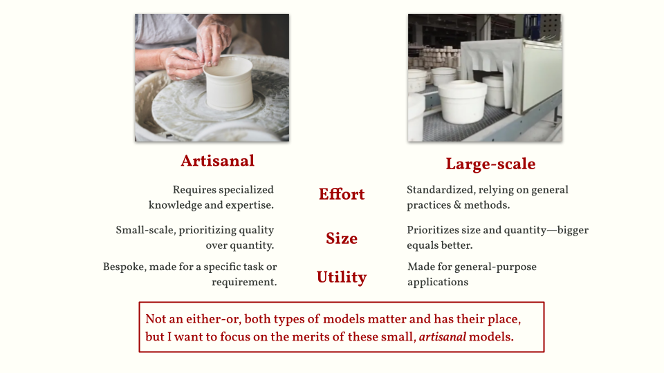
In this talk, I want to contrast two types of ideas when building language technologies. You have artisanal on one end, as shown by this photo of a handmade pottery—carefully constructed by its creator. On the other hand, you have these “mass-produced” objects done in large-scale. I want to differentiate them in terms of three dimensions.

1. Effort: artisanal NLP resources often require specialized knowledge and effort. For example, it is important to know something about Filipino grammar and morphology when building task-specific models for Filipino. Large-scale models can get away with just providing large amounts of data (as we see in most web-scale datasets).

2. Size: currently, our definitions of what’s small or large change every month. But in general, artisanal models are relatively smaller in terms of parameter size. Large-scale models need to be bigger because they have to accommodate more tasks and domains.

3. Utility: artisanal models and datasets tend to be bespoke, i.e., built for a specific task or requirement. On the other hand, most large-scale models we see today were made for general-purpose applications.

Notice that I’m a bit vague whether I’m talking about models or datasets. I like to think of artisanal vs. large-scale as an attitude for building language technologies or NLP artifacts. Finally, this talk is not about one being better than the other. However, I want to focus more on the merits of these artisanal NLP resources by discussing parts of my research and my work.

You can see the outline of my lecture below. For the rest of this talk, I’ll fill the blanks and talk about the merits of artisanal NLP while discussing portions of my research.

Artisanal NLP resources are high-effort, but impactful for the language community

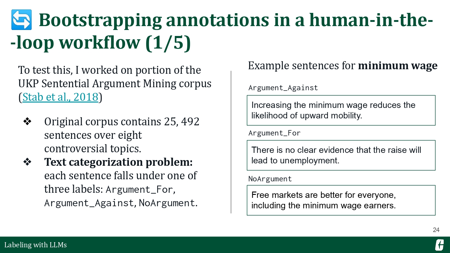
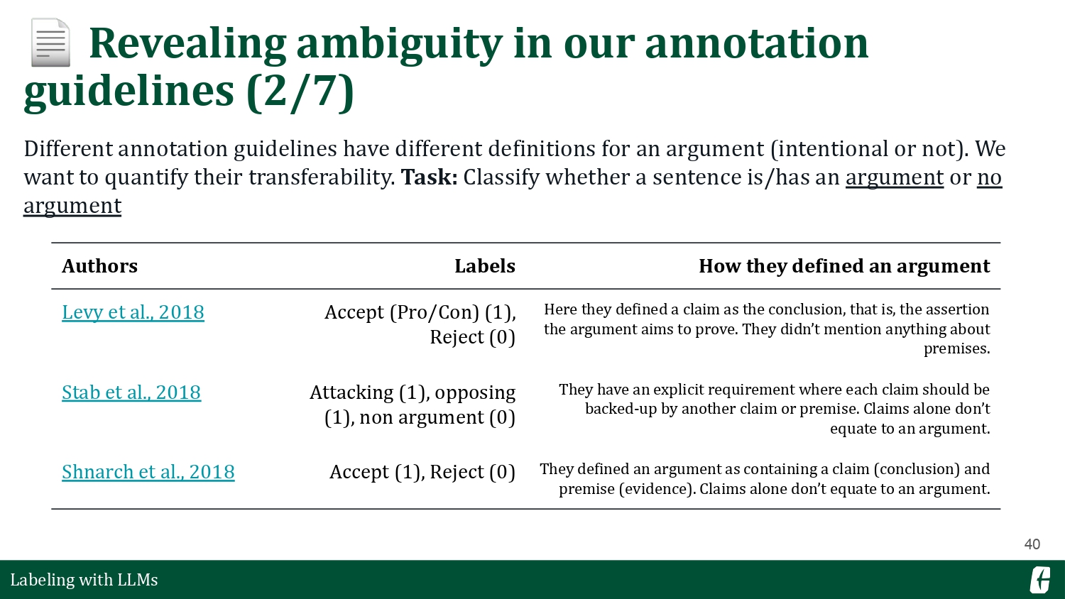
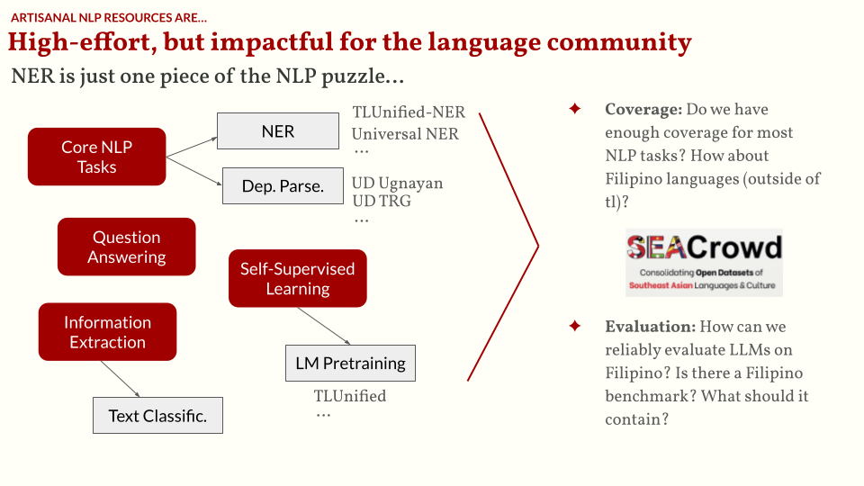
In this section, I want to talk about TLUnified-NER (link to SEALP ‘23 paper), a Named-Entity Recognition dataset that I’ve built. NER is a classical NLP problem: given a text, you want to look for named-entities such as names of persons, locations, or organizations.

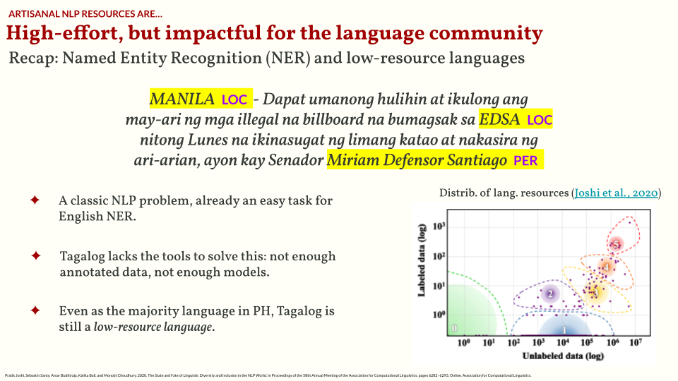
This is already an easy task for English NER. However, NER resources for Tagalog are still lacking. We don’t have a lot of labeled data, and in consequence we don’t have a lot of models. There are many ways to get around this problem (e.g., cross-lingual transfer learning, zero-shot from an LLM), but we still lack reliable test sets for evaluation.

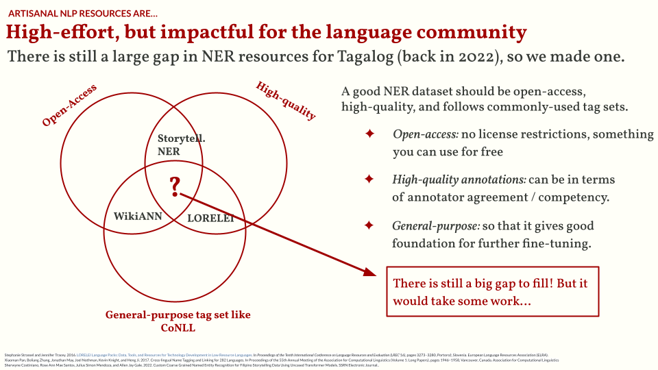
In my opinion, a good NER dataset should be open-access, high-quality, and standardized. Most of the NER datasets available for us only fills two of these three attributes: WikiANN has general-purpose tags that follow CoNLL and can be downloaded from HuggingFace, but the quality of annotations are pretty bad. LORELEI is a high-quality dataset, but has strict license restrictions and quite expensive! Finally, we have several hand-annotated datasets for Filipino, but most of them were made for highly-specific tasks. Back in 2022, there’s an obvious gap to fill for Tagalog NER.

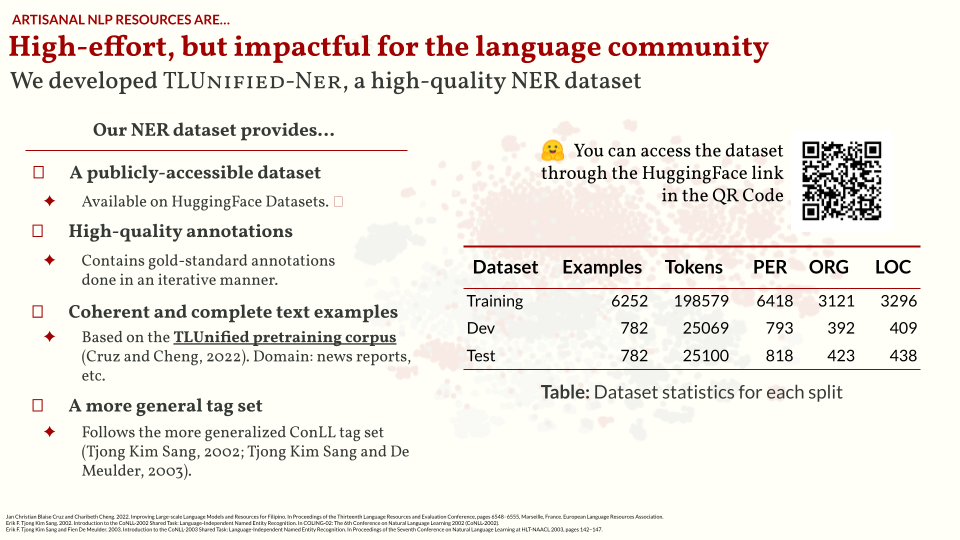
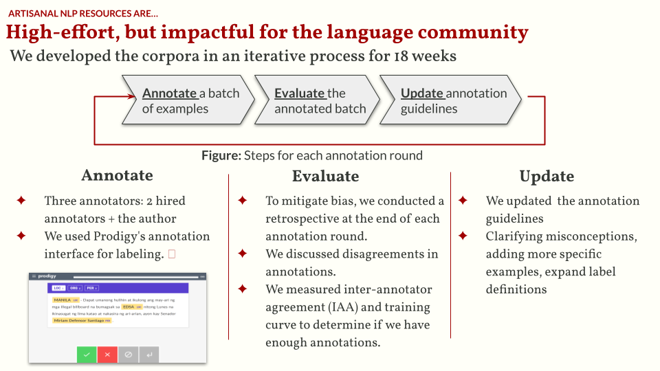
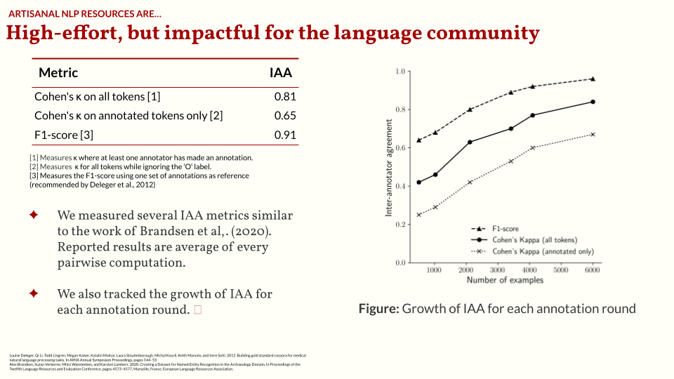
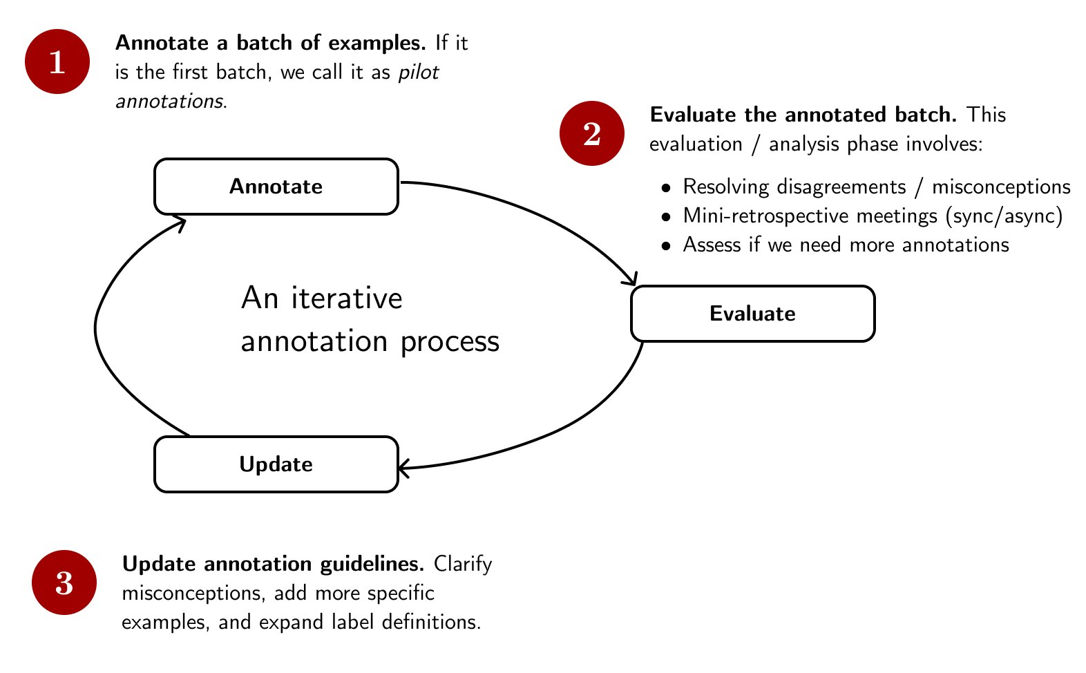
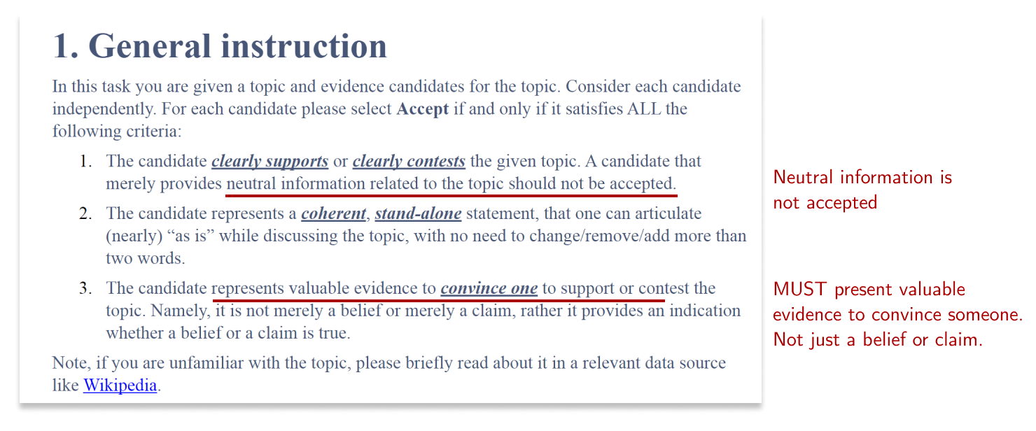
And so we built TLUnified-NER. It is publicly accessible, high-quality, and follows the CoNLL standard. I also curated the texts to ensure that it represents how we commonly write Tagalog. The annotation process is done through several rounds (or sprints). I hired two more annotators and then for each round we annotate a batch of examples, evaluate the annotated batch, and update the annotation guidelines to improve quality. You can learn more about this process in our paper. I also wrote some of my thoughts on the annotation process in a blogpost.

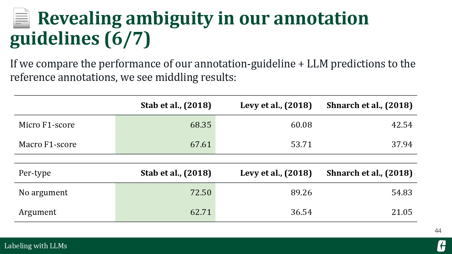
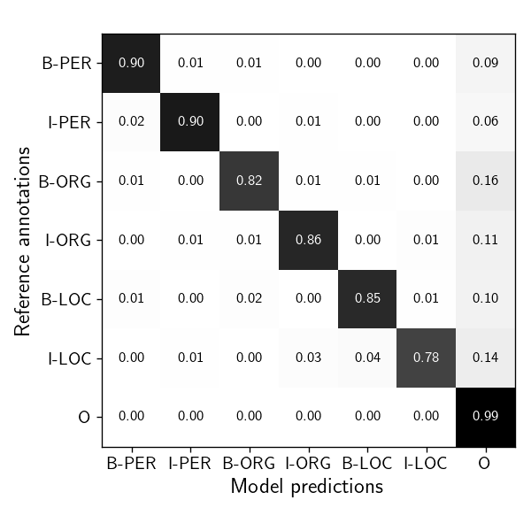
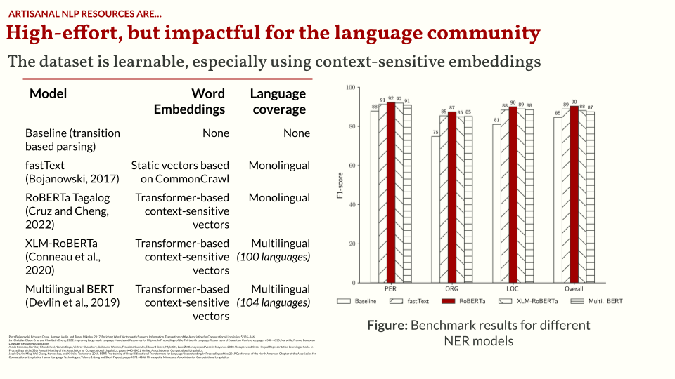
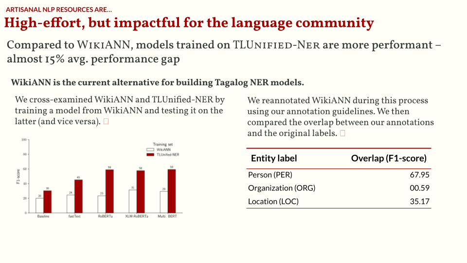
After building the dataset, there are two questions that I want to answer: first, is the NER task learnable from our annotations? Then, is it better than existing NER datasets? For the first one, I created baseline approaches using various mixes of word embeddings and language coverage. For all cases, we achieved decent performance. Then for the second question, we compared a model trained on WikiANN and a model trained from TLUnified-NER. In most cases, our model outperforms the WikiANN model, showing that it’s a better dataset to train models upon.

To end this part of the talk, I want to show that NER is just one piece of the NLP puzzle. There are still a lot of tasks to build resources on. I believe that increasing the coverage of Filipino resources allows us to not only train models, but create comprehensive evaluation benchmarks for existing LLMs today. Recently, we’ve seen a lot of claims that LLMs can “speak” Filipino, but most of these are cherry-picked examples and highly vibes-based. If we can create a systematic benchmark that allows us to confidently claim performance, then that would be a big contribution to the field.

Artisanal NLP resources are capable of doing a few things, but can do them well

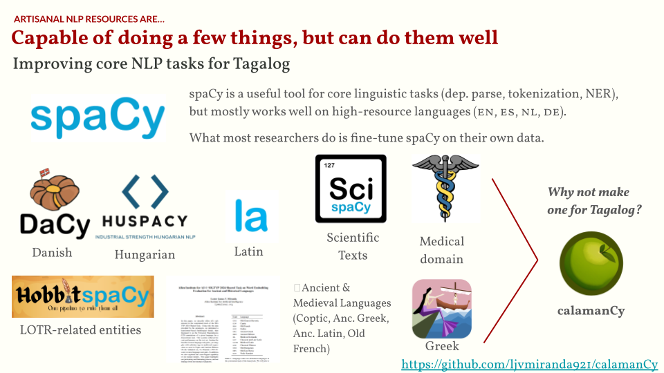
In this section, I’ll talk about calamanCy, a spaCy-based toolkit that I built for Tagalog (NLP-OSS ‘23 paper). As you already know, spaCy is a toolkit for core linguistic tasks such as dependency parsing, tokenization, and NER. However, most of the models we provide in-house are focused on high-resource languages.

What most people do is they finetune spaCy pipelines on their own language or domain. So you’ll see libraries in the spaCy universe for all kinds of applications.

So this prompted me the question: why don’t we build a spaCy pipeline for Tagalog?

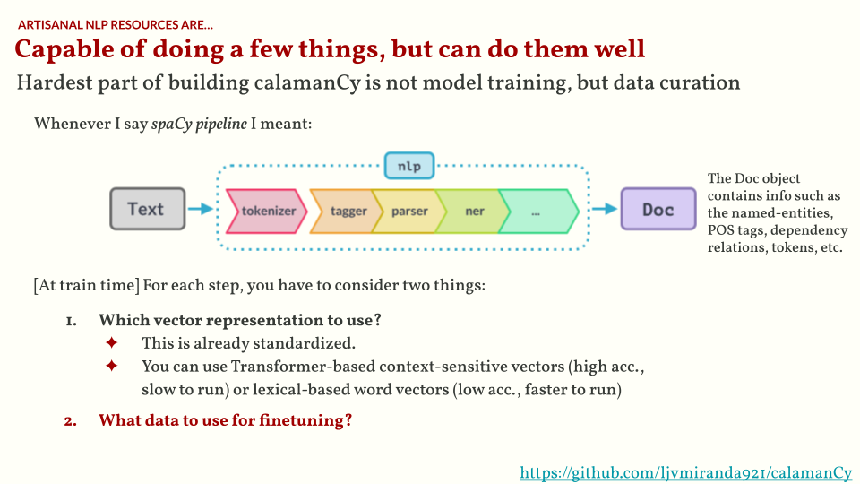
But what does it mean to build spaCy pipeline?

First, think of a spaCy pipeline as a series of functions that identifies key linguistic features in a text. So a tokenizer is a function that looks for tokens, a tagger is a function for parts-of-speech (POS) tags, and so on. Then at the end, you obtain a Doc object that contains all these linguistic features.

Building a spaCy pipeline means training these functions and composing them into a single package. In fact, we have a well-documented master thread on how to add pretrained language support for spaCy. Most of these functions are based on neural network architectures, and hence require some non-trivial amount of data to train.

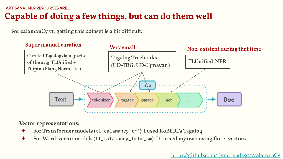
One of the hardest parts of building calamanCy is curating datasets to “train” these functions. For example, the current Tagalog treebanks are too small to train a reliable dependency parser and POS tagger. Also, TLUnified-NER doesn’t exist back then, so I still have to build it. You can read more about this curation process in the calamanCy paper.

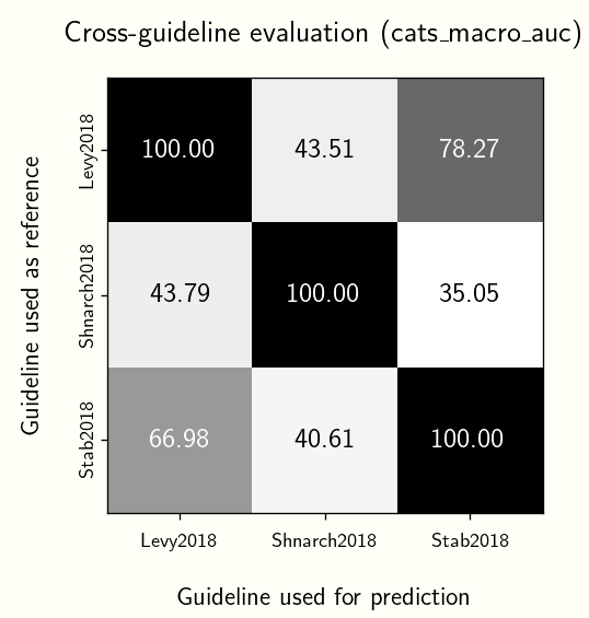
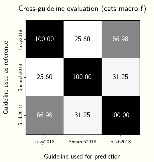
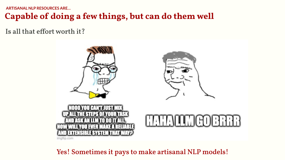
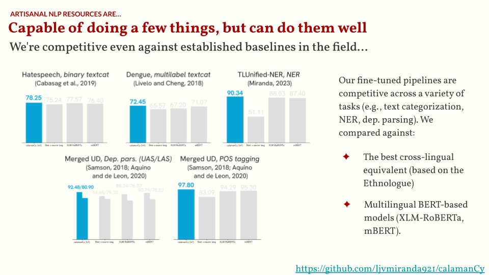
It was a long process, but the most important question is: was it worth it? To that I remember this figure from Matthew Honnibal’s blog post on LLM maximalism. I think there is value in curating these datasets and training these models as it helps me understand which parts of the linguistic pipeline really requires an LLM, and which could be done more reliably by a simple approach. In addition, we were also able to show empirically that models trained on calamanCy performs pretty well, even compared to commercial LLM APIs.

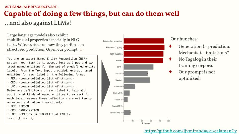
As shown in the charts below, we found that even commercial LLMs like GPT-4 and Claude don’t fare well on our test set in a zero-shot setting. There are many possible reasons, of course. One major reason is that these models aren’t optimized for multilinguality, and hence have a tiny amount of Tagalog texts in their corpora. I’d love to revisit this experiment soon, especially with the release of multilingual LLMs such as SeaLLM, Sea-LION, and Aya-101.

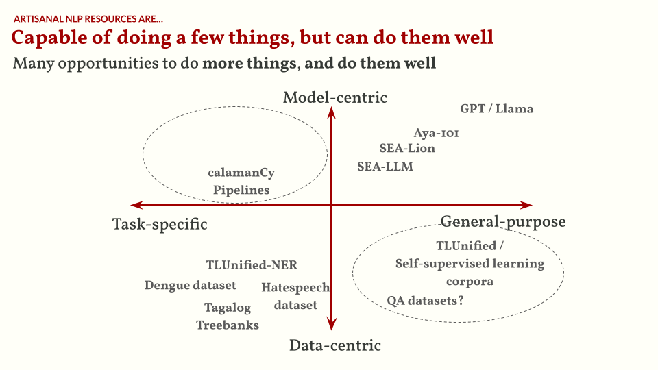
So…even if artisanal NLP models can do a few things (but do them well), I’m still optimistic that there are opportunities to do more things while doing them well. I want you to remember this chart below. There are a lot of opportunities to work on datasets used for training models with general-purpose capabilities and/or building task-specific models.

Artisanal NLP resources may not be the most mainstream, but fills vital research gaps

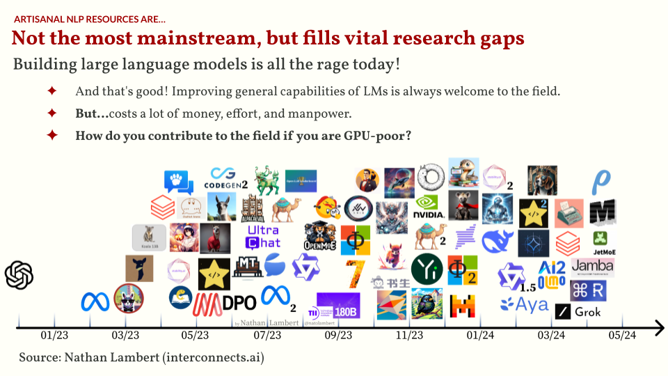
As we all know, LLMs are all the rage today. In the past two years, there has been an explosion of open LLMs, and way more soon! However, working on LLM research is costly— a high-spec consumer-grade machine might not be enough to finetune a 7B-parameter model. So how do you contribute to the field if you are GPU-poor?

I will answer this in the context of my collaborations and other works.

The first option is to continue building resources, but at scale. It’s quite common to see researchers first work on a single language (mostly that of their native tongue) and then move on to multilinguality, as the latter presents a different opportunity for creativity.

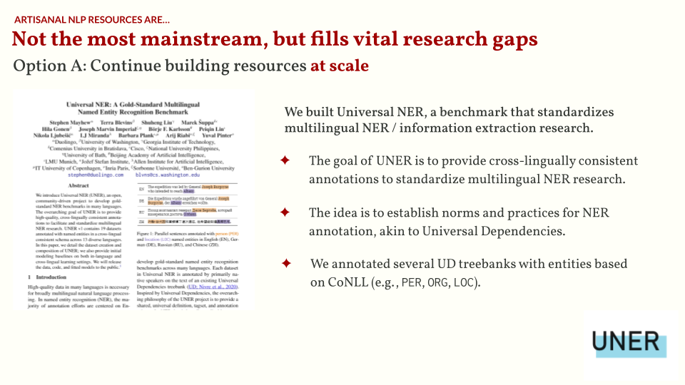
For Universal NER, we created a multilingual NER corpora for several languages, all based from treebanks in the Universal Dependencies (UD) framework. This effort allows us to create a consistent and standardized annotation for 13 diverse languages— very important for multilingual research.

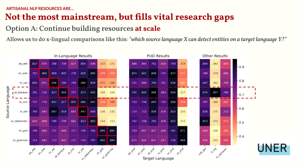
As an illustration, we can do cross-lingual transfer learning as shown below, where we compare the performance of different models trained on a source language for different test set languages. We can even show that for low-resource languages like Tagalog, we can get by with training an NER model from a Portuguese treebank as an alternative.

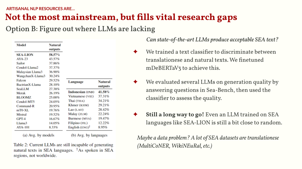
Another option is to figure out areas where LLMs are lacking. Most LLMs right now aren’t explicitly trained to be multilingual. They’re incidentally multilingual, probably because of some stray artifacts in their pretraining data. But for the past few months, we’ve seen the rise of multilingual LLMs such as Aya-101, Sea-LION, and more. Are they actually better for multilingual data?

That’s one of the questions we sought to answer in the SEACrowd project. First, we crowdsourced datasets all over Southeast Asia. This allows us to create a data hub for SEA-specific resources. The data hub, in itself, is already a big contribution. It also allowed me to see available datasets from the Philippines, and there’s actually quite a lot!

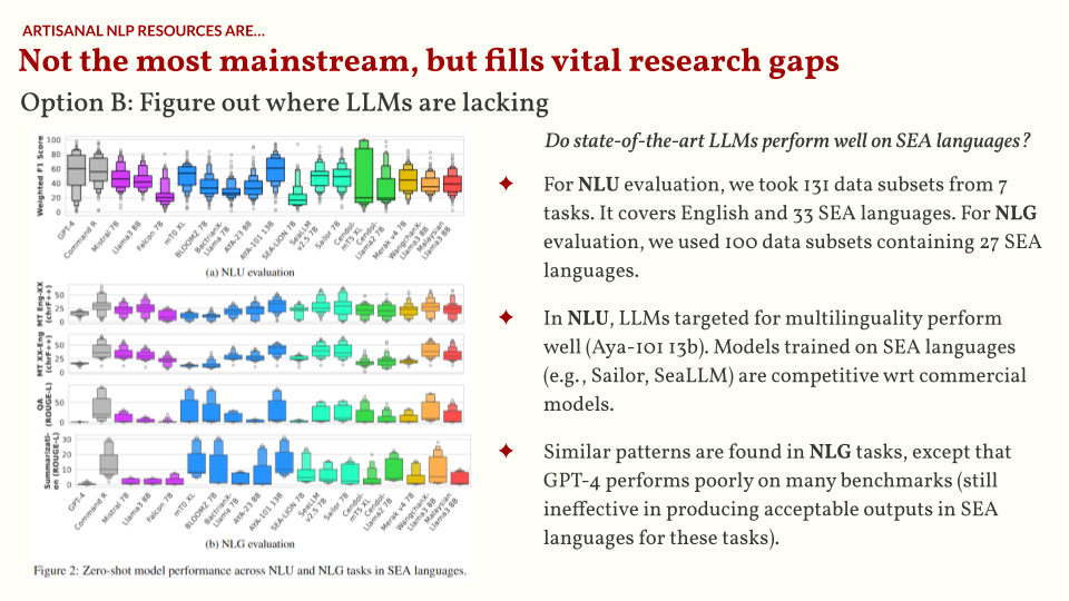
Then, we curated a multilingual SEA benchmark for both NLU (natural language understanding) and NLG (natural langauge generation) tasks. Upon testing, we found that LLMs trained for multilinguality actually perform quite well (e.g., Aya-101 13B). Even LLMs targeted for SEA languages are competitive with commercial APIs.

What I found very interesting is that when testing for generation “quality” (i.e., are the generated texts natural-sounding or translationese?), we found that even the best LLM is still 58% natural-sounding. There’s still a long way to go to improve the quality of generations. As of now, everything is still vibes-based, but having an empirical benchmark certainly helps!

Conclusion: what types of artisanal NLP contributions can you pursue?

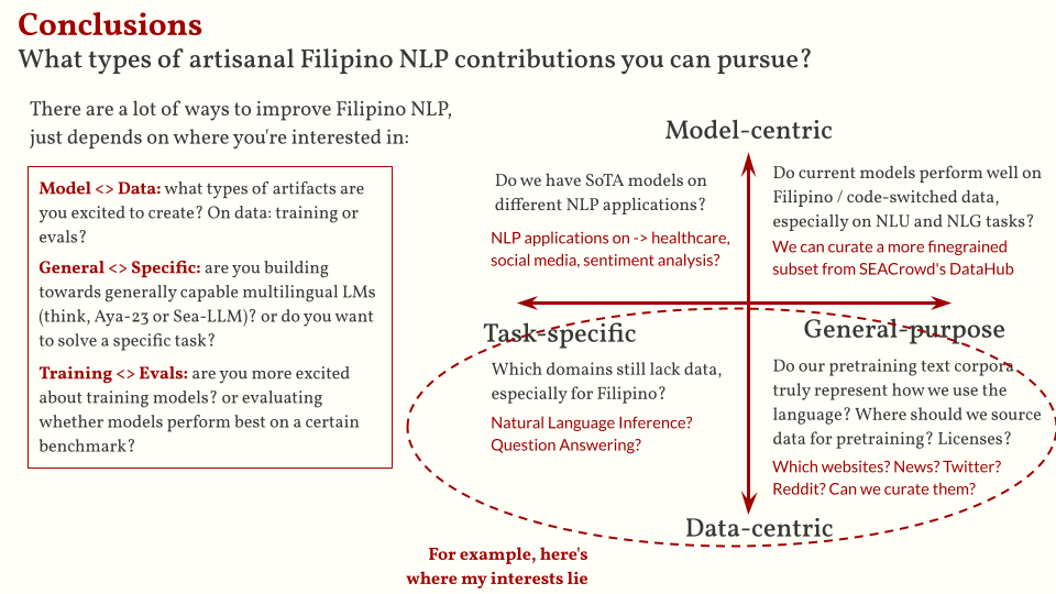
I want to close this talk by showing you this chart. There are a lot of ways to improve Filipino NLP, it just depends on where you’re interested in:

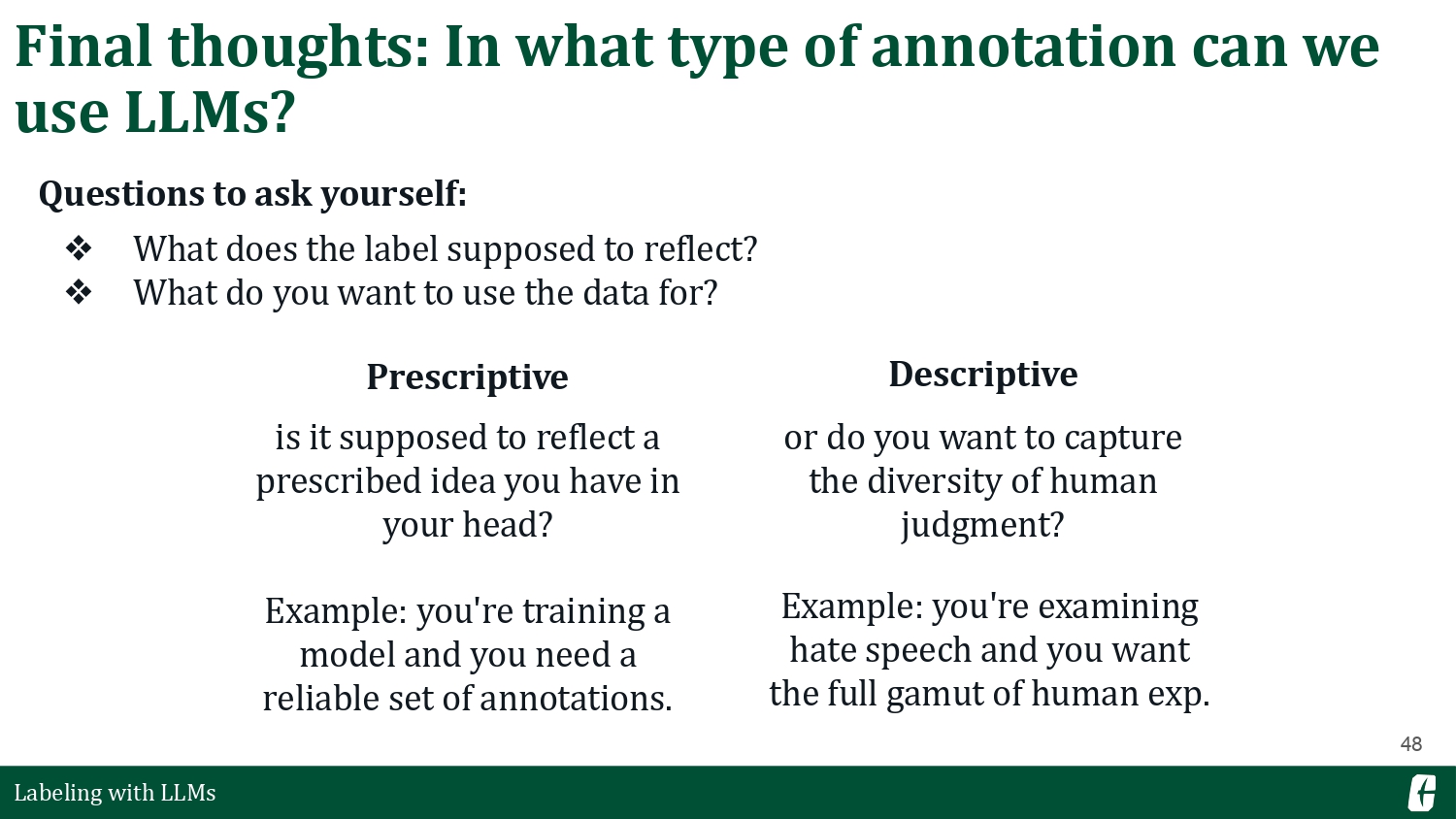
• Model-centric or data-centric: what types of artifacts are you excited to build? Do you want to curate datasets or do you want to build models?
• General-purpose or specific: are you aiming to build towards generally-capable LLMs, or do you want to solve a specific task?
• Training or evals: what is the purpose of the artifact you’re creating? Is it for training models or for evaluating existing models?

There are opportunities for each quadrant of this chart. I myself am interested in data-centric approaches for both task-specific and generally-capable models. There’s still a lot of domains that need foundational NLP resources (think Universal Dependencies treebanks), and several questions can still be asked regarding the datasets we use for training state-of-the-art LLMs.

Hopefully this inspires you to figure out what your project would be!

Postscript

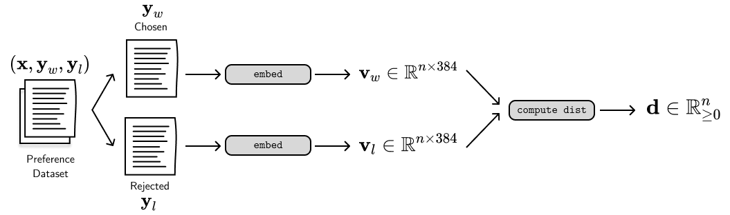
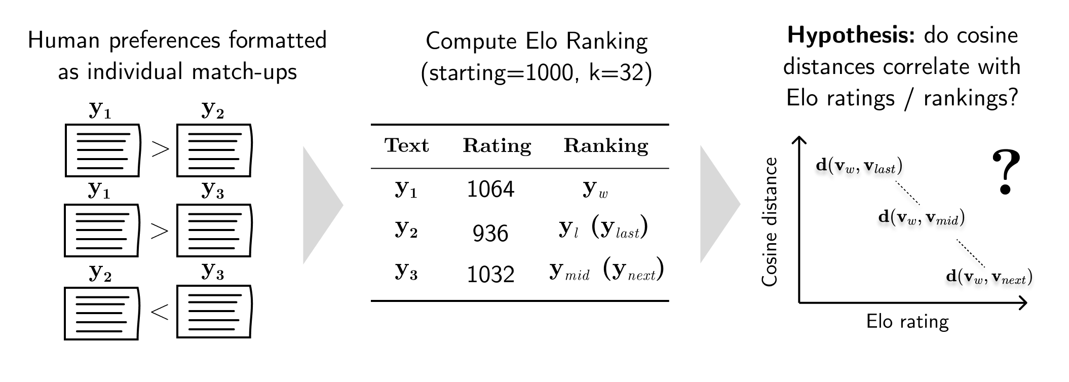
I really enjoyed preparing for this talk as it helped me synthesize my past work on Filipino NLP. Right now, I’m finding ways to marry my current research (preference / alignment-tuning for LLMS) and my previous work on low-resource and multilinguality. I’m quite inspired by works such as the PRISM Alignment Project, Cohere’s Aya-23 dataset, and the Multilingual Alignment prism. I think there are interesting questions at the intersection of multilinguality and preference data, but I don’t think our conclusions should be something like “Oh, people who speak language X prefers Y and Z” or “People from country A prefers B.” Still a long way to go, but I’m excited to pursue these topics in the future! If this caught your attention, feel free to reach out!

However, preference is subjective by nature, and few studies have tried articulating it. For example, some looked into different aspects of a response’s helpfulness / harmlessness (Bai et al., 2022) while others investigated surface-level characteristics like its length (Singhal et al., 2023).

In this blog post, I want to offer a different approach: what if instead of looking at qualitative aspects or token-level features, we use sentence embeddings? Sentence embeddings capture a text’s lexical and semantic meaning in a high-dimensional vector space. If so, can we ascertain lexical differences between chosen and rejected responses just by looking at text embeddings?

One reason why this is important is due to synthetic data. I think that it is easier to generate synthetic pairs conditioned on lexical distance (as opposed to some quality-based metric). Maybe, there are some tasks and domains where generating with respect to cosine distances is plausible.

Getting preference data

First, I sampled preference data across different sources. For bigger datasets such as SHP, I only took a particular subset I am interested in. The table below shows the sources I used:

For OpenAI’s Summarize and SHP, the preferences are in the form of individual matchups. To get the canonical chosen and rejected responses, I used the Elo rating system to obtain the top and bottom completions.

Measuring distance between pairs

Given a set of preference data, I split the completions based on whether they were chosen (\(\mathbf{y}_w\)) or rejected (\(\mathbf{y}_l\)) by an evaluator—human or GPT, depending on the dataset. Then, I embedded them using sentence-transformers/all-MiniLM-L6-v2 to produce 384-dimensional sentence embeddings. Finally, for each row, I computed the distance (\(\mathbf{d}\)) between the chosen and rejected vectors. The figure below illustrates this process.

To compute the distances, I used the cosine distance from scipy. Cosine distance measures the direction between two vectors, allowing us to capture similarity even if the length of the sentences or overall frequency of the words differ. It is represented by the following equation:

where the distance value ranges from \((0, 2)\). Usually, when we talk about distances between preference pairs, we talk about quality-based distances. They’re often in the form of rankings (i.e., get top-1 and top-N) based on an evaluator’s assessment. Again, in this blog post we’re looking at lexical-based distances that are readily available from a text’s surface form. In the next section, I’ll discuss some interesting findings from these distance calculations.

Findings

Most of the charts I’ll be showing below are histograms. Here, the x-axis represents the cosine distance whereas the y-axis represents the probability density. We compute the probability density by normalizing the fraction of samples in each bin so that the sum of all bar areas equals 1. The best way to think about these value is in terms of chance, that is, how likely is a random preference pair have a distance \(\mathbf{d}\) on the x-axis?

Lexical differences are apparent in some datasets

The chart below shows the distribution across multiple preference datasets. AlpacaFarm and Nectar lie on both extremes. AlpacaFarm is particularly interesting because its completions were generated by API-based LLMs using prompts that replicate human variability and agreement. I’m unfamiliar with how exactly they prompted the LLM, but does that mean their process resulted in similar-looking texts?

On the other hand, Nectar’s completions were a combination of LLM outputs (GPT-4, GPT-3.5-turbo, GPT-3.5-turbo-instruct, LLaMa-2-7B-chat, and Mistral-7B-Instruct) alongside other existing datasets. Because Nectar formats its preferences in terms of ranking, the chosen and rejected pairs here represent the top and bottom choices.

Other datasets have distributions that I expected. For example, OpenAI’s summarization dataset should still have closer preference pairs because of the task’s inherent nature. Summarization is about compressing a text while maintaining information. Upon checking the actual preferences and corresponding evaluator notes, I noticed that rejected completions are oftentimes a matter of recall.

Elo ranking correlates with cosine distance

Next, I looked into how Elo ranking corresponds to the cosine distance of the text embeddings. Preference datasets like OpenAI’s Summarization, SHP, and Berkeley-Nest’s Nectar represent their preferences as individual matchups, allowing us to compute the Elo rating of individual completions. Then, we can order these ratings to achieve a rank of completions from most preferable to least.

However, OpenAI’s Summarization and SHP have unequal number of ranks per prompt \(\mathbf{x}\). So to simplify the visualizations, I took the chosen completion \(\mathbf{y}_w\), the top-2 completion \(\mathbf{y}_{l,next}\), the middle-performer \(\mathbf{y}_{l,mid}\), and the bottom-performer \(\mathbf{y}_{l,last}\) (which is equivalent to \(\mathbf{y}_l\) in the previous section). On the other hand, Berkeley-Nest’s Nectar provides a 7-rank scale of preferences. This allowed me to compute the distance from the first and second choices until the last one: \(\mathbf{d}(\mathbf{y}_1, \mathbf{y}_{2\ldots7})\). Then, I plotted these distances in a histogram (I only retained the curve so that the charts look cleaner) as seen below:

The cosine distances from the OpenAI Summarization preference dataset follow a certain pattern: completions that are closer in ranking have smaller lexical distance. The average mid ranking is 2.042 (with a 4.109 average number of ranks) and the Pearson correlation between the distances and Elo ranking is 0.779.

For the Stanford Human Preferences (SHP) dataset, I chose the explainlikeimfive subset to simulate OpenQA tasks. Interestingly, it has a less pronounced visual correlation even though its Pearson-r is 0.785, much higher than OpenAI Summarization. The average mid ranking is 1.967 with an average rank number of 4.600.

For Berkeley-Nest’s Nectar dataset, the rankings were already given so I didn’t have to compute my own. Here, the Pearson correlation is 0.818. If you look at the “chosen and rejected (2)” red line, you’ll notice that the cosine distances start very small but fall off afterwards. It is interesting that completions that performed similarly during matchups are quite similar to one another based on their embeddings.

The table above shows the ranking statistics for each dataset. I also measured the Pearson correlation between the rejected text’s ranking (and Elo rating) with respect to its embedding distance from the chosen text. The sign (+/-) corresponds to the direction of the correlation. For example, the negative sign in the last column shows that as the text’s Elo rating increases, then its lexical distance from the chosen text decreases (i.e., they become more similar).

Lexical distance is consistent across preference attributes

Finally, I was curious how individual attributes of preference manifest in lexical distances using the HelpSteer dataset (Wang et al., 2023). Most datasets only give us a single view of human judgment, but HelpSteer provides finegrained preferences such as helpfulness, correctness, coherence, complexity, and verbosity.

So, I did the same experiments for each of these attributes and found that the distribution didn’t change much. I’m not quite confident on how I preprocessed this dataset. Unlike other preference datasets that uses matchups, HelpSteer uses scores from 0 to 4 so some texts can end up having the same scores. Here, I simply sorted the texts with their score, and designated the chosen text as the first one on the list (whatever Python’s sort function made it to be), and the rejected text as the last element. You can see the figure below:

I think that there’s still a lot that can be done on this angle. One way is to format the data in terms of individual matchups. This process leads to a forced ranking, allowing us to easily designate the chosen and rejected pair. Since HelpSteer is the only one we have (as far as I know), then I’ll leave my analysis as is for now.

Final thoughts

In this blog post, I presented a lexical view of preference pairs using embeddings. Using different preference datasets, I computed for their sentence embeddings, and then measured the cosine distance between chosen and rejected pairs. I found that some datasets exhibit lexical differences and that it correlates to human judgment (i.e., Elo rating). Finally, using the HelpSteer dataset, I saw that cosine distances are consistent even on different attributes of preference.

This experiment is really just a curiosity as I work on RLHF. I’ve been doing some experiments on my job that are a little bit orthogonal to this work. I think this is just my way of exploring interesting avenues and scratching my itch. If you’re interested in this type of work, feel free to reach out and discuss!

You can find the source code for this work on GitHub!

This blog post is my (abridged) lecture in written format. You can find the slides in this link. Finally, thanks to Ryan Wesslen and Chang Hsin Lee for inviting me!

Case in point: automated fact checking

One of the major problems of the 21st century is disinformation. You’ll see it everywhere, from Facebook posts or X tweets to fake news websites! Combating disinformation is labor-intensive. Politifact, a fact-checking website, relies on volunteer journalists to scour the internet and manually label each source.

There are several efforts to automate the fact-checking process. A common approach is to treat it as an NLP pipeline composed of different tasks (Guo et al., 2022). Today, we will only focus on claim detection, the first step in an automated fact-checking pipeline.

Detecting claims is usually a dual problem: you’d also want to find the premises that support it. Together, the claim and its premises make up an argument. Applying NLP to this domain is often called argument mining. For this talk, I want to introduce two argument mining sub-tasks: (1) first, we want to highlight the claim and premise given a text (claim & premise extraction), and then, (2) we want to determine if a text supports, opposes, or is neutral to a certain topic (stance detection).

So, our general approach is to reframe these two sub-tasks as NLP tasks. First, we treat claim & premise extraction as a span labeling problem. We can use spaCy’s SpanCategorizer to obtain spans or arbitrary slices of text. Then, we treat stance detection as a text categorization problem. Similarly, we can use spaCy’s TextCategorizer to classify a text among our three stances (support, oppose, neutral).

Notice how we’ve decomposed this general problem of disinformation into tractable NLP tasks. And it is an important muscle to train. In computer science, we often learn about the divide and conquer algorithm, and this is a good application of that approach to a more fuzzy and, admittedly, complex problem.

As we already know, training NLP models such as a span or text categorizer requires a lot of data. I want to talk about different methods of collecting this dataset and emphasize how LLMs can fit into this workflow.

Annotating argument mining data with LLMs

Before we get into LLMs, I want to talk about “traditional” ways of annotating data. On the left end, we have manual processes involving much human effort and curation. And then, on the right, we have more automated methods that rely heavily on a reference or base model. LLMs, as advanced as they are, still fall in between. They’re not fully manual but also not fully automated because writing a prompt still requires tuning and domain expertise.

But why are we still interested in LLMs? It’s because LLMs provide something that most semi-automated methods can’t: a model pretrained on web-scale data, and a highly flexible zero-shot capability. Let me put this in a Venn diagram— and for each space in this diagram, I’ll talk about how LLMs can specifically help in our annotation workflows.

Bootstrapping in a human-in-the-loop workflow

One of the most straightforward applications of large language models is bootstrapping labeled data. Here, an LLM is a drop-in replacement for a base model that you’d usually train. LLMs differ because they were pretrained on web-scale data, giving it enough capacity even for your domain-specific task. So, how good is an LLM annotator?

To test this question, I worked on a portion of the UKP Sentential Argument Mining corpus (Stab et al., 2018). It contains several statements across various topics, and the task is to determine whether the statement supports, opposes, or is neutral to the topic— a text categorization problem.

The process was simple: I included each statement in a prompt and asked GPT-3.5 what the stance was. You can read more about my process in this blog post. My findings show that LLMs, when prompted in a zero-shot manner, are competitive on a baseline that I trained on the original labels. In addition, I also found myself annotating faster (and more correctly) when correcting LLM annotations compared to annotating from scratch. The latter finding is important because correcting annotations induces less cognitive load and human effort (Li et al., 2023, Zhang et al., 2023).

So, if LLMs can already provide competitive annotations, is our problem solved? We don’t have to annotate anymore? Remember, the reason why we collect these annotations is so that we can train a supervised model that can reliably approximate the task we’re interested in. The operating word here is reliable. There’s a huge variance in LLM performance, and one way to thin out that curve is to insert it in a human-in-the-loop workflow (Dai et al., 2023; Boubdir et al., 2023; Wang et al., 2023).

Directing annotations by providing extra info in the UI

Another way we can use LLMs for annotation is by taking advantage of their flexibility. LLMs have zero-shot capabilities, i.e., we can always frame structured prediction tasks such as text categorization or named entity recognition as a question-answering problem. Back then, you’d need to train separate supervised models to achieve multi-task skills. I want to use an LLM’s flexibility to enhance the annotation experience.

This time, I want to introduce two workflows. The first one is still a text categorization problem, but I want to ask an LLM to pre-highlight the claims and premises so I can reference them during annotation. For the second one, I want to ask the LLM to do the reasoning for me. I’ll let it identify the claims and premises, then pre-annotate an answer, and then give me a reason for choosing that answer. This exercise aims to explore creative ways we can harness LLMs.

The process is similar to the first section, but I prompt for auxiliary information instead of prompting for the direct labels. LLMs make this possible because we can formulate each task as a question-answer pair. You’ll find examples of my prompt in the slides below. The prompt on the left is a straightforward span labeling prompt, where we ask the LLM to provide the exact spans from a text. On the other hand, the prompt on the right is a chain-of-thought prompt (Wei et al., 2023). Here, we induce an LLM to perform a series of reasoning tasks to arrive at a final answer.

The good thing about Prodigy is that you can easily incorporate this extra information in your annotation UI. On the bottom left, you’ll see that it highlights the claims and premises for each statement, allowing you to focus on the relevant details when labeling. On the bottom right, you’ll find that the UI metadata now contains the prompt’s reasoning steps.

There are many creative ways to improve annotation efficiency (and quality) using LLMs. One of my favorite papers from EMNLP was CoAnnotating (Li et al., 2023), which uses an uncertainty metric to allocate annotation tasks between humans and a chat model such as ChatGPT. We’ve seen a lot of LLM-as-an-assistant applications in the market for the past year, and I think that there’s an opportunity to apply the same perspective to the task of annotation.

Revealing ambiguity in our annotation guidelines

Finally, I’m curious how LLMs parse information originally intended for humans. In most annotation projects, researchers write an annotation guideline to set up the parameters of the labeling task. These guidelines aim to reduce uncertainty about the phenomenon we are annotating. We can even think of these as prompts for humans!

This time, I want to focus on a simple task: determine whether a statement is an argument. It sounds easy because it’s “just” a binary classification task. However, after looking through various argument mining papers and their annotation guidelines, I realized that they each have their definition of what makes an argument!

So, this got me thinking: what if we include the annotation guideline in the prompt? You can check my entire experiment in this blog post. Back then, you could not fit a whole document into an LLM’s limited context length, so I used a continuous prompting strategy that showed chunks of the document and let the LLM update their answer based on new information. Langchain calls this a “refine chain” in their docs. As an aside, I’ve opted into using minichain in my recent projects as it is more lightweight and enough for my needs.

Including an annotation guideline in the prompt resulted in worse results—surprising. I couldn’t delve further, but I hypothesize that writing prompts for LLMs have a particular “dialect” vastly different from how we talk as humans. Annotation guidelines were written with humans in mind, and perhaps some qualities don’t transfer properly into LLM prompts. There are many confounding factors, of course. Maybe the refine strategy is not the best, or maybe I should’ve processed the text much better. An LLM’s prompt sensitivity is still an open problem.

But I learned one thing: we can use LLMs as a “first pass” when iterating over our annotation guidelines. Typically, you’d start with a pilot annotation with a small group of annotators as you write the guidelines, but there’s an opportunity to incorporate LLMs into the mix.

Final thoughts

Before we end, I want to share an important question before you begin your annotation projects. You should always ask yourself: what is the label supposed to reflect? Knowing what you want to use the collected dataset for is paramount.

Rottger et al. (2022) named two paradigms for data annotation: prescriptive and descriptive. Prescriptive annotation is usually found in linguistic tasks such as named entity recognition or parts-of-speech tagging—where there is a “correct” answer for each instance. Here, you already have a function in mind and need to collect enough data to train a reliable model. On the other hand, descriptive annotation aims to capture the whole diversity of human judgment. You’d usually find this in subjective tasks like hate speech detection or human preference collection.

LLMs are pretty good at prescriptive annotation tasks. Some empirical evidence that supports it (Ashok et al., 2023; Chen et al., 2023; Sun et al., 2023), and it allows us to access the web-scale data it was pretrained upon.

And now to my final point: despite their web-scale and zero-shot capabilities, LLMs are only as good as how well you prompt them. During my early days in data science, there is this common adage: “garbage in, garbage out.” Usually, we say this when we want to refer to bad data. The problem with prompts is that the degree of freedom is much higher, which introduces ambiguity to our inputs. Hence, I don’t recommend using LLM outputs straight from the firehose and serving it immediately. There should be an intermediary step that minimizes this uncertainty, and that step is human annotation.

$ git clone git@github.com:myorg/repo.git
Cloning into 'repo'...
ERROR: The 'myorg' organization has enabled or enforced SAML SSO.  
To access this repository, you must use the HTTPS remote with a 
personal access token or SSH with an SSH key and passphrase that 
has been authorized for this organization.

Visit https://docs.github.com/articles/authenticating-to-a-github-organ
ization-with-saml-single-sign-on/ for more information.

Step 1: Create an SSH key and upload it to your GitHub account

First you need to generate your SSH key. Sometimes, your organization will require you to generate a new one using your company email. Nevertheless, the common denominator would be to run the ssh-keygen command below:

ssh-keygen -t ed25519 -C lj@myorg.org

This will generate a key pair in the form of id_ed25519 and id_25519.pub. In Linux, you can find them in the ~./ssh/ directory. We need to upload the one with the .pub extension to GitHub. Go to your GitHub Settings > SSH and GPG Keys > New SSH Key (or head to github.com/settings/keys).

Write a semi-descriptive title (I usually put the organization name), set the Key Type as “Authentication Key,” and copy the contents of the id_25519.pub in the Key field.

Step 2: Add your SSH key to the SSH agent’s list

First, test the connection by running:

$ ssh -T git@github.com
Hi username! You've successfully authenticated, but GitHub does 
not provide shell access.

Then, start the SSH agent:

$ eval "$(ssh-agent -s)"
Agent pid 16935

It starts a background daemon and displays its process ID (in this case, 16935). We can then add our private keys while this agent is running.

$ ssh-add .ssh/id_ed25519
Identity added: .ssh/id_ed25519 (some other info)

At this point, you should now be able to clone your organization’s private repository. I haven’t really dug deep as to why it errored out the first time, I assumed that the keys are automatically added whenever I create them. Anyway, in case you also encountered this error, I hope this tutorial helps!