Training a neural network using differential evolution
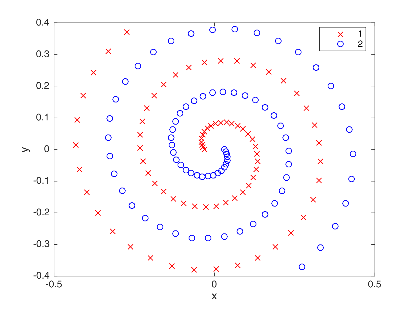
This is a simple implementation of a 2-16-1 neural network trained using Particle Swarm Optimization in order to solve the two-spiral problem. The \(\sin(z)\) and \(\sigma(z)\) activation functions were used for the input-hidden and hidden-output layers respectively. The cross-entropy error was used as the cost function. The two-spiral problem is a particularly difficult problem that requires separating two logistic spirals from one another (Lang and Witbrock, 1998).
Differential Evolution
As a member of a class of different evolutionary algorithms, DE is a population-based optimizer that generates perturbations given the current generation (Price and Storn, 2005). But instead of generating vectors using samples from a predefined probability functions, DE perturbs vectors using the scaled difference of two randomly population vectors.
Differential Evolution produces a trial vector, \(\mathbf{u}_{0}\), that competes against the population vector of the same index. Now, once the last trial vector has been tested, the survivors of the pairwise competitions become the parents for the next generation in the evolutionary cycle.
Methodology
For Differential Evolution, a three step process will be done. First, we will initialize the population, set-up the optimization system, and then tune the hyperparameters. Initialization will be based from a Gaussian distribution, while the tuning will involve the mutation and recombination parameters.
Our neural network simply consists of one hidden layer with a \(sin(x)\) activation function (Sopena, Romero, et al., 1999).
Initialization
For any particle \(n = 1,2, \dots , N\), its position \(P\) at time-step \(t\) with respect to the ANN parameters are expressed as:
\[P_{n,t} \equiv \begin{bmatrix} \Theta_{11}^{(1)} & \Theta_{12}^{(1)} & \dots & \Theta_{ij}^{(1)}\\ \Theta_{11}^{(2)} & \Theta_{21}^{(2)} & \dots & \Theta_{jk}^{(2)} \end{bmatrix}\]The particle matrix P was initialized using uniform distribution. This is to maximize the exploration capability of the particles over the search space by distributing it evenly. Using a Gaussian distribution to initialize the particles will “scatter” it in a centered weight , reducing the exploration capacity.
Optimization System
-
Mutation: For mutation, three random vectors are chosen, and relate them in order to produce the donor vector ,\(v_{i,G+1}\). This method is controlled by the parameter \(F\) (\(F \in [0,2]\)). The equation for producing the donor vector is \(v_{i,G+1} = x_{r1,G} + F (x_{r2,G} - x_{r3,G})\)
-
Recombination: For recombination, the trial vector is built using the elements of the donor vector (donorVec) and the elements of your target vector. This means that for each particle in the population (for each row of particle) and for each dimension of that particle (for each column of each row of particle), a comparison is made with respect to the parameter \(CR\).
-
Selection: For selection, the target vector is then compared against the trial vector if the fitness value is less than the computed fitness of the target, then that particle is replaced with the one captured from the trial vector. After all particles are tested, we then have the second generation.
Implementation Parameters
| Parameter | Description |
|---|---|
genMax |
Number of generations that the DE algorithm will run |
population |
Number of particles in the search space. |
epsilon_de |
Scattering degree of the particles during initialization |
mutationF |
Degree of mutation effect (exploration parameter) |
recombinationC |
Degree of recombination effect (exploitation parameter) |
Tuning the mutation and recombination parameters
Here, I swept over different values of \(m\) and \(c\) in order to find good values for my final model.
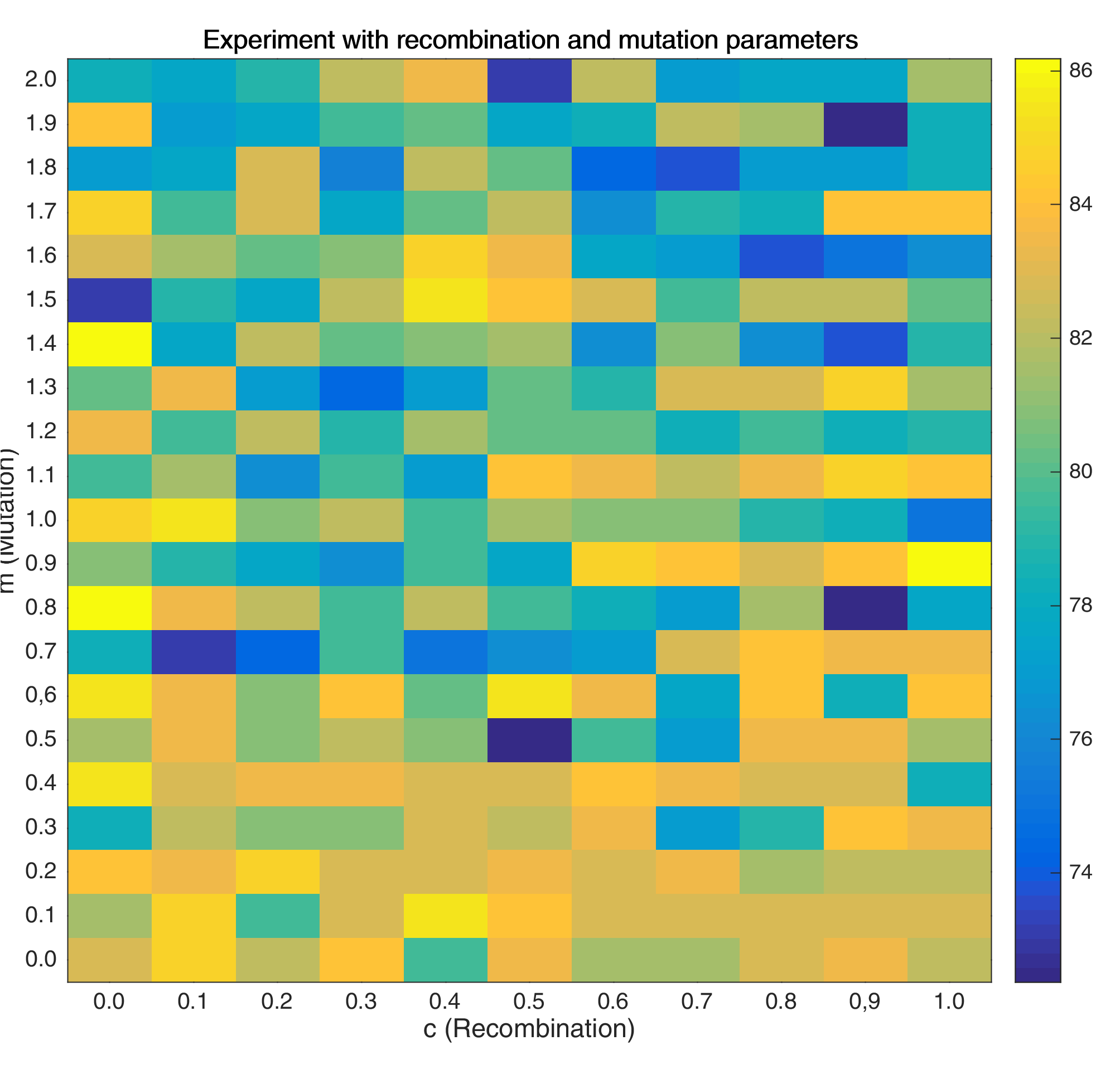
As shown, it may be better to use lower mutation values coupled with very low recombination values.
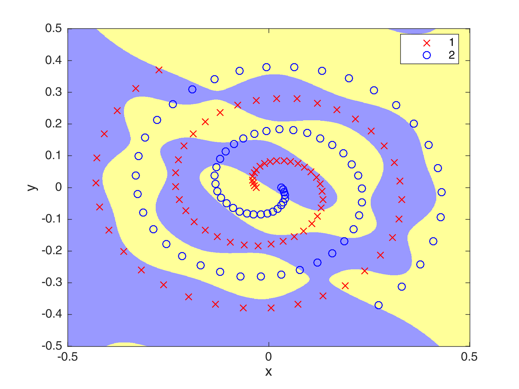
Results:
The best score that was achieved using this optimization algorithm is 84.8684% recall. The figure below shows the generalization ability that the algorithm can attain. Moreover, the table below shows the values I set for the parameters.
| Parameter | Value |
|---|---|
genMax |
5,000 |
population |
20 |
epsilon_de |
0.1 |
mutationF |
0.19 |
recombinationC |
0.07 |
Conclusion
Using the differential evolution to train a neural network is much faster as compared to PSO. However, one problem with PSO is on how the production of a completely new generation is affected by the population size \(N\). Because each vector is being replaced one by one, it may also require \(N\) iterations in order to fully replace the current generation and find a more suitable candidate solution.
In terms of performance, DE and PSO’s best solutions are not really that far apart. Although these values are achieved in different iterations, i.e., DE needing more time to get to converge to a better solution. In my opinion, it is also possible to modify the DE algorithm by taking into consideration the gradient produced by backpropagation. This gradient may be used as a scale to “mutate” the donor vector, thus making the mutated vectors much better. Although this gradient needs to be modified so that the stochastic element is still present.
References
- J. M. Sopena, E. Romero, and R. Alquezar. 1999. Neural Networks with Periodic and Monotonic Activation Functions: A Comparative Study in Classification Problems. In Proceedings of the Ninth International Conference on Artificial Neural Networks (ICANN).
- Kevin J. Lang and Michael J. Witbrock. 1988. Learning to Tell Two Spirals Apart. In Proceedings of the 1988 Connectionist Models Summer School.
- Kenneth V. Price, Rainer M. Storn, and Jouni A. Lampinen. 2005. Differential Evolution: A Practical Approach to Global Optimization. Springer. Implementation gist: \urlhttps://gist.github.com/ljvmiranda921/53939299b9e67f0df082e0127c7f229d.