Training a neural network using particle swarm optimization

This is a simple implementation of a 2-16-1 neural network trained using Particle Swarm Optimization in order to solve the two-spiral problem. The \(\sin(z)\) and \(\sigma(z)\) activation functions were used for the input-hidden and hidden-output layers respectively (Sopena, Romero, et al., 1999). The cross-entropy error was used as the cost function. The two-spiral problem is a particularly difficult problem that requires separating two logistic spirals from one another (Lang and Witbrock, 1998).

Figure 1: Graph of the Two-Spiral Problem

Particle Swarm Optimization

Particle swarm optimization is a population-based search algorithm that is based on the social behavior of birds within a flock (Engelbrecht, 2007). In PSO, the particles are scattered throughout the hyperdimensional search space. These particles use the results found by the others in order to build a better solution.

Methodology

For Particle Swarm Optimization, we first initialize the swarm, and then observe the effects of the social and cognitive parameters to its performance. After that, parameter tuning will be implemented as the neural network will be cross-validated with respect to the social and cognitive parameters.

Initialization

For any particle \(n = 1,2, \dots , N\), its position \(P\) at time-step \(t\) with respect to the ANN parameters are expressed as:

\[P_{n,t} \equiv \begin{bmatrix} \Theta_{11}^{(1)} & \Theta_{12}^{(1)} & \dots & \Theta_{ij}^{(1)}\\ \Theta_{11}^{(2)} & \Theta_{21}^{(2)} & \dots & \Theta_{jk}^{(2)} \end{bmatrix}\]

The particle matrix P was initialized using uniform distribution. This is to maximize the exploration capability of the particles over the search space by distributing it evenly. Using a gaussian distribution to initialize the particles will “scatter” it in a centered weight , reducing the exploration capacity.

Implementation Parameters

Parameter	Description
maxIter	Number of iterations that the PSO algorithm will run
swarmSize	Number of particles in the search space.
epsilon	Scattering degree of the particles during initialization
c_1	Cognitive component (exploration parameter).
c_2	Social component (exploitation parameter).
inertiaWeight	Inertia weight that controls the movement of particles.

Table 1: Parameters used in PSO Implementation

Tuning the social and cognitive behaviour of the swarm

Here, I swept over different values for the social and cognitive components, and came up with this matrix:

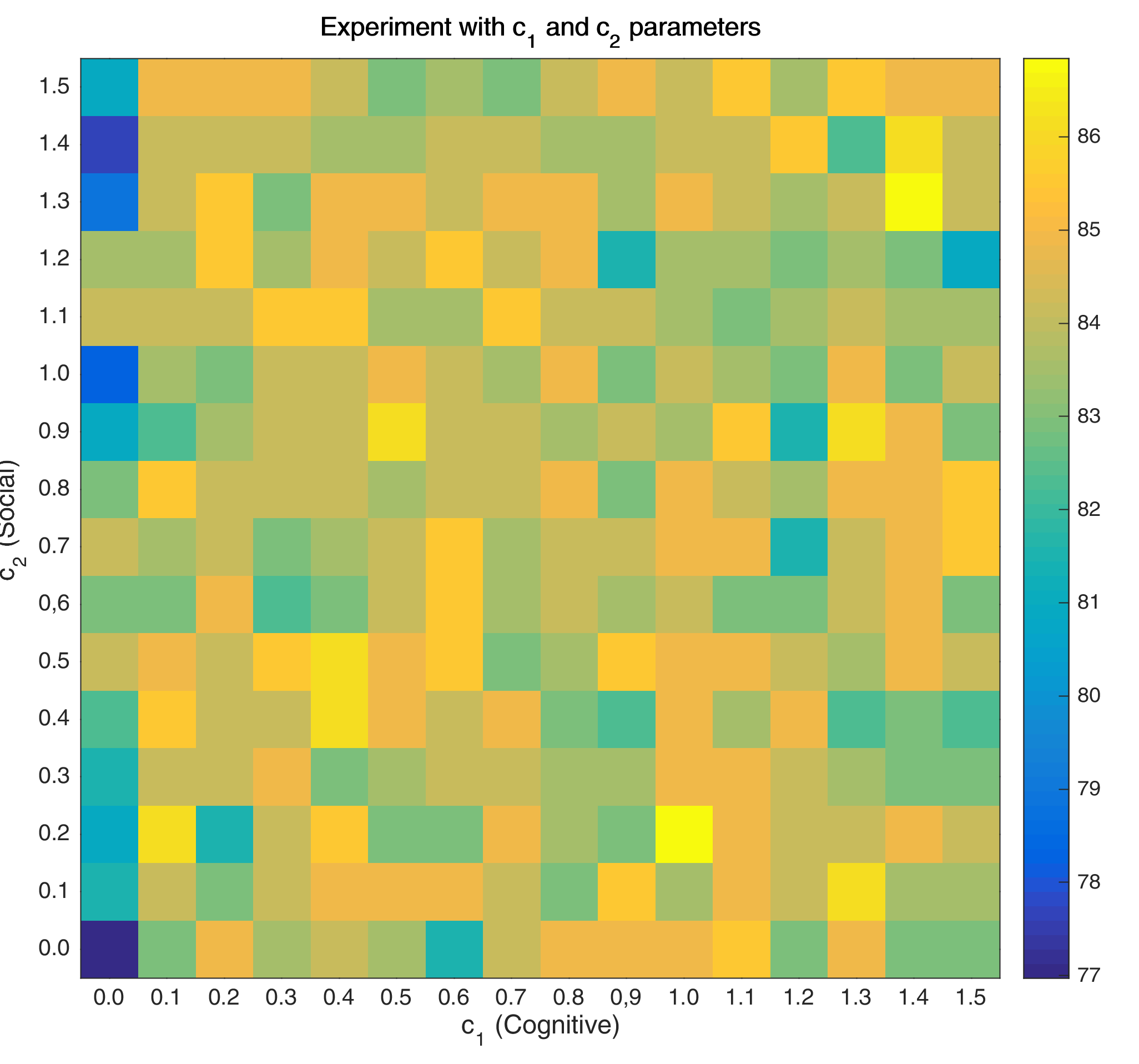
Figure 2: Heat map for testing the social and cognitive parameters

From this value matrix, it is clear that accuracy may improve with values where the ratio of \(c_{1}\) and \(c_{2}\) is \(\approx 1\). Moreover, it also shows that setting a very low cognitive value doesn’t improve the solution. However, because the value matrix doesn’t give anything definitive regarding the settings for \(c_{1}\) and \(c_{2}\), a more heuristic approach is applied.

Observation of Swarm Behavior

The following images below show the simulation of the swarm (only at parameters \(\theta_{11}^{(1)}\) and \(\theta_{12}^{(1)}\)) given different values of the social and cognitive components. Below these simulations, a graph of the cost is traced. One can then see the differences in their behavior by looking on the convergence of the “mean best” with respect to the personal and global bests.

Figure 2: Swarm behavior at when it is fully social (left) and fully cognitive (right)

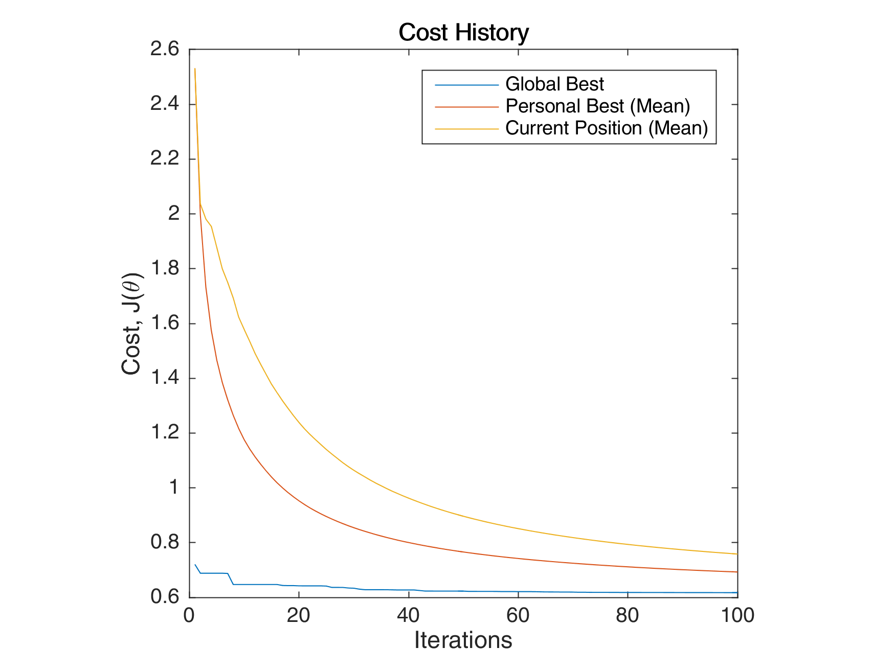
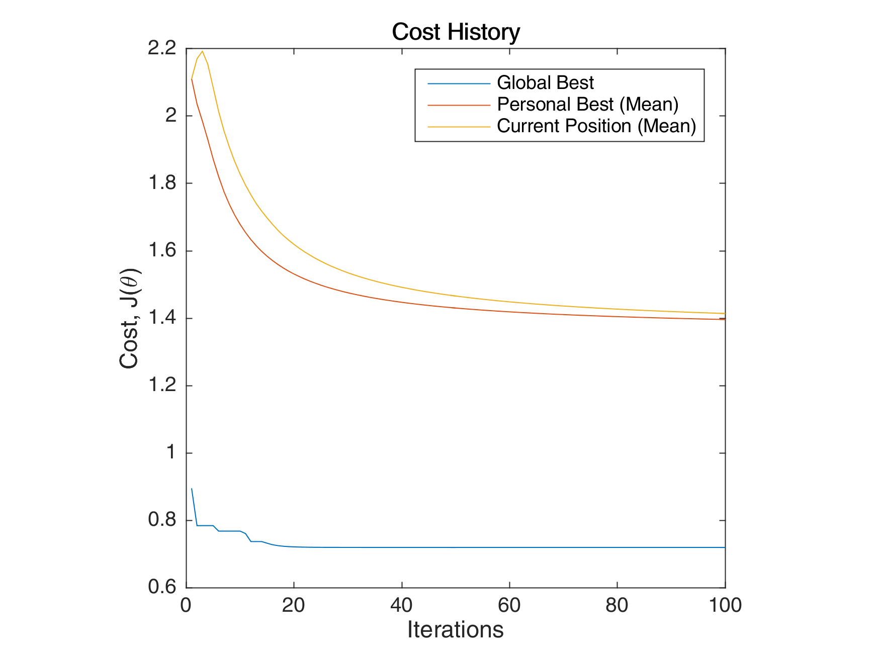
Figure 3: Graph of the cost per iteration

For a swarm that has no cognitive parameter, the particles tend to move to the global best quite early, resulting to a curve that converges easily. On the other hand, for a swarm that has no social parameter, the particles tend to move only to their personal bests, without doing an effort to reach the best score found by the whole swarm.

Results

The best score that was achieved using this optimization algorithm is 85.5264% recall. The figure below shows the generalization ability that the algorithm can attain. Moreover, the table below shows the values I set for the parameters.

Parameter	Value
maxIter	200
swarmSize	50
epsilon	0.1
c_1	1.5
c_2	0.9
inertiaWeight	0.7

Table 2: Parameter values for PSO Implementation

Figure 4: Generalization ability of the PSO-trained Neural Network over the whole space

Conclusion

One of the main advantage of PSO is that there are only (at a minimum) two parameters to control. Balancing the tradeoff between exploitation and exploration is much easier as compared to other algorithms because it is much more intuitive. However, initialization is also important in PSO. It matters how the particles are distributed along the search space as it may increase or decrease their chances of finding the optimal solution. In this implementation, a small value of \(0.1\) was used for the spread parameter \(\epsilon\).

Compared with the benchmark solution, the PSO has a tendency to run slower. Moreover, as the number of particles increase, the computational time increases because the size of the matrices to be computed also expands. This problem may be solved using advanced vectorization techniques in MATLAB, but overall, the PSO runtime often correlates with the swarm size.

References

• Engelbrecht, Andres (2007). Computational Intelligence: An Introduction, John Wiley & Sons.
• Sopena, J.M., Romero, E. and Alquezar, R. (1999). “Neural networks with periodic and monotonic activation functions: a comparative study in classification problems”. In: ICANN Ninth International Conference on Artificial Neural Networks.
• Lang, K.J. and Witbrock, M.J. (1988). “Learning to Tell Two Spirals Apart”. In: Proceedings of the 1988 Connectionist Models Summer School

You can access the gist here.