Study notes on making word vectors from scratch
Word vectors are representations of words into numbers. Once words are in this form, it becomes straightforward for a computer to understand them. Of course, you can’t just arbitrarily assign numbers into words!
We need to satisfy two conditions: first, is that these numbers should have some meaning, or semantics. Second, is that we should encode meaning into a numerical representation. If we’re in the realm of numbers, a common way to show meaning is to see how far one number is from another:

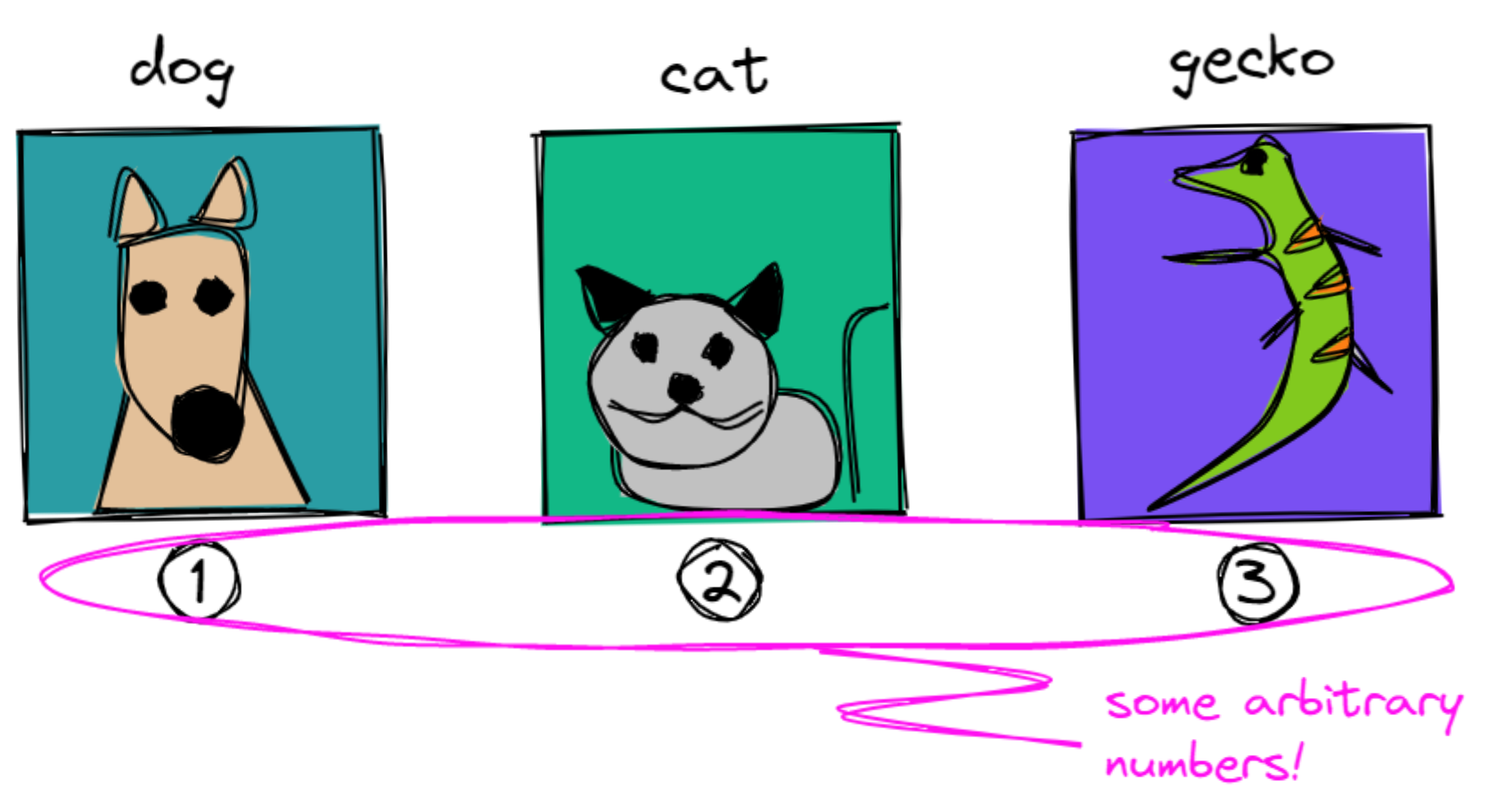
The hope is, words can also be represented as such. In the case of animals, one trait, or feature, that we can encode is its leggedness. Let’s plot our animals on a number line depending on the number of their legs:
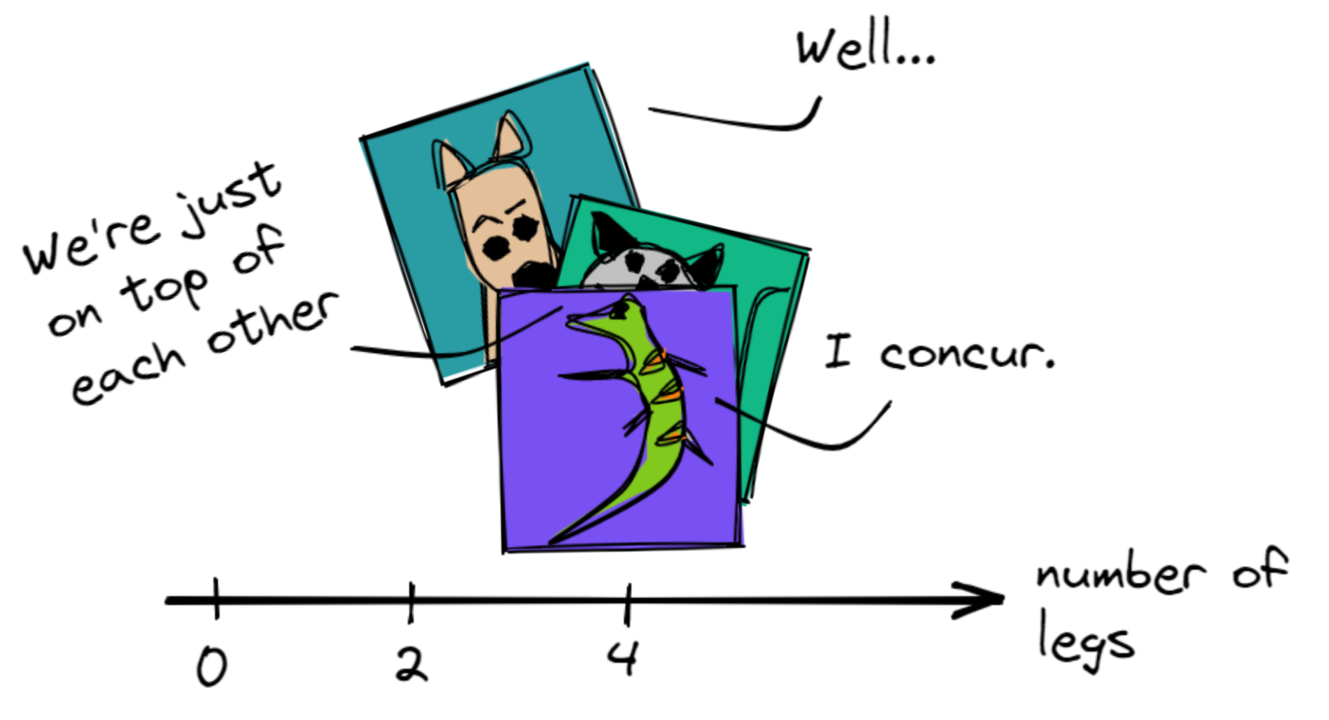
That’s not yet informative, all the animals were stacked on top of each other. Perhaps we can add another feature, how about tameness? Let’s create another axis and place our animals across them:
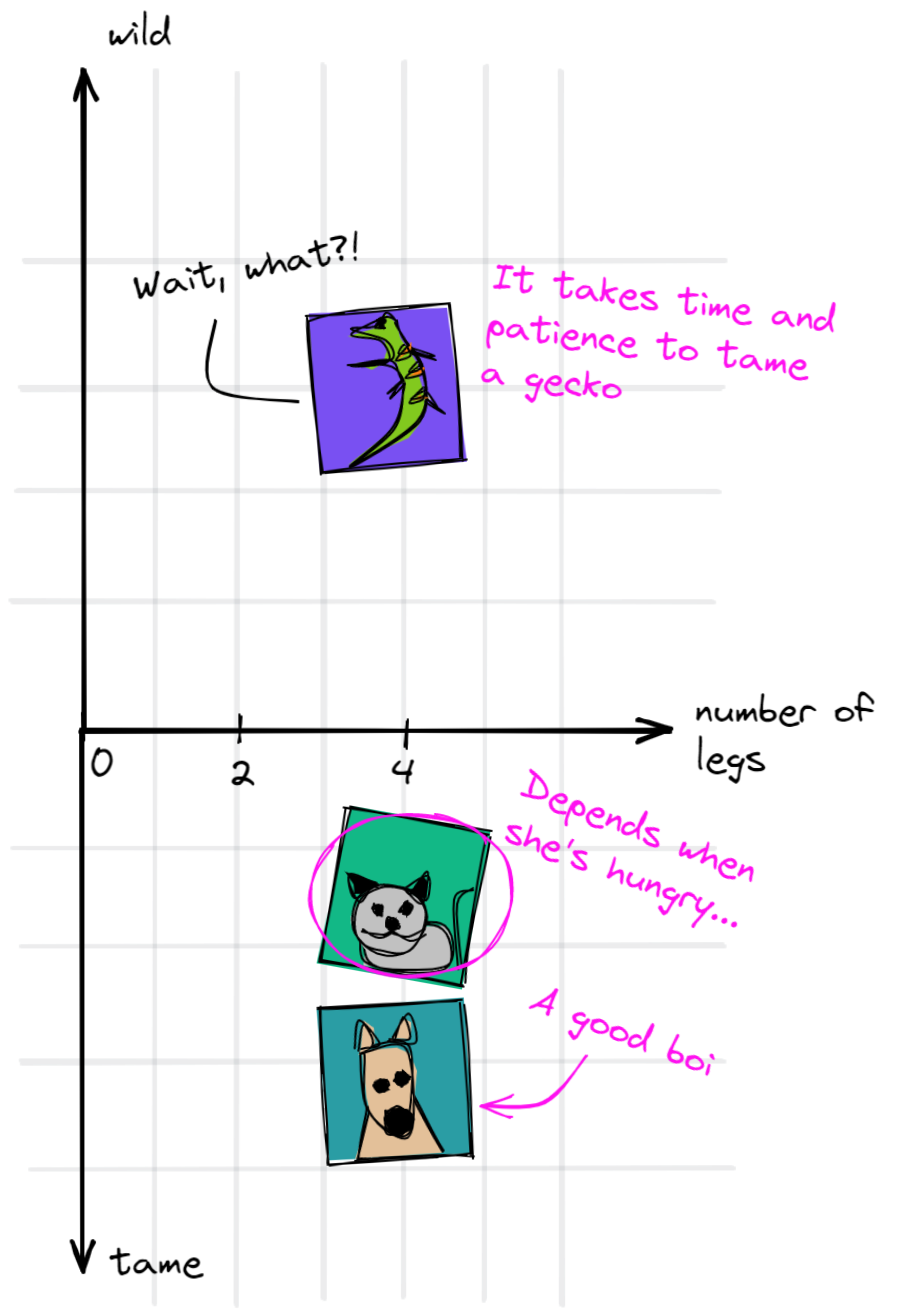
What we just did is that we came up with features and encoded them into our vectors. As a result, we can now say that a dog is similar to a cat, entirely different from a gecko, and so on.
But we don’t want to write all possible features one-by-one, we want to exploit existing knowledge just for that. We also don’t want to encode them manually, we’d rather write an algorithm to automate that for us.
This gives us to two ingredients in creating word vectors:
- An existing corpus of knowledge to get features automatically. Here, we can use newspaper clippings, scraped data from the web, scientific journals, and more!
- An encoding mechanism to transfom that text into numbers. Instead of writing them manually, we encode it algorithmically.
Contents
Word vectors from scratch
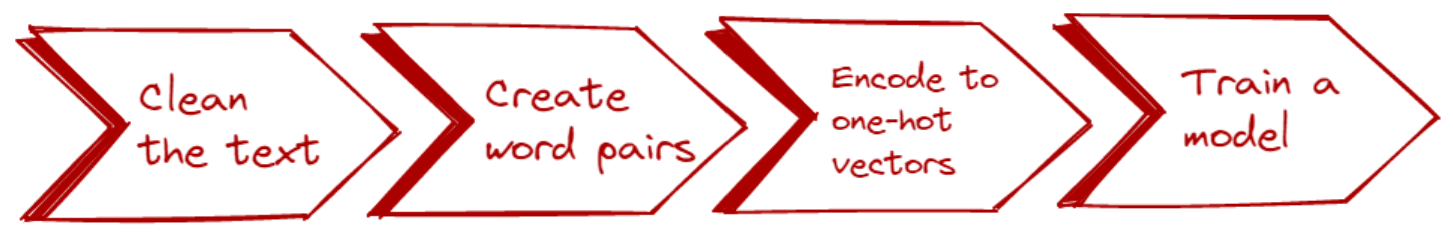
We’ll use these two ingredients— the corpus and encoding algorithm— to create word vectors from scratch. Some of these were adapted from this blogpost. We’ll start from a small text corpus and end with a set of word vectors. The process is as follows:
0. Preliminary: the text corpus 📚
Earlier, we manually encoded our knowledge into some mathematical format. When we spoke of tameness, we assigned values to each of our animals and plotted them into the graph. This method is great if you only deal with one or two features. But when you want to capture the nuance and meaning ascribed to those words, it’s not enough.
In practice, we extract knowledge from other sources: books, the Internet, Reddit comments, Wikipedia, and more.
In practice, we’d want to extract knowledge from other sources—books, the Internet, Reddit comments, Wikipedia…you name it! In NLP, we call this collection of texts as the corpus.1 We won’t be scraping any text for now. Instead, we’ll come up with our own:
sentences = [
    "A dog is an example of a canine",
    "A cat is an example of a feline",
    "A gecko can be a pet.",
    "A cat is a warm-blooded feline.",
    "A gecko is a cold-blooded reptile.",
    "A dog is a warm-blooded mammal.",
    "A gecko is an example of a reptile.",
    "A mammal is warm-blooded.",
    "A reptile is cold-blooded.",
    "A cat is a mammal.",
]
What you see above are factual statements about animals. Think of them as a sample of sentences you’ll typically find in any corpus. In reality, ten sentences aren’t enough to generate a good model, you’d want a larger corpus for that. For example, the GloVe word embeddings used Wikipedia, news text, and the Internet (CommonCrawl) as its source. It has hundreds of gigabytes of data, a million times more than the ten sentences we have.
1. Clean the text 🧹
We clean the texts by removing stopwords and punctuations. In NLP, stopwords are low-signal words that are uninformative and frequent.2 A few examples include articles (a, an, the), some adverbs (actually, really), and a few pronouns (he, me, it).
Most libraries like spaCy, nltk, and gensim provide their own list of stopwords. For us however, we’ll stick to writing our own:
STOP_WORDS = [
    "the",
    "a",
    "an",
    "and",
    "is",
    "are",
    "in",
    "be",
    "can",
    "I",
    "have",
    "of",
    "example",
    "so",
    "both",
]
We also write our own blacklist of punctuations:
PUNCTUATIONS = r"""!()-[]{};:'"\,<>./?@#$%^&*_~"""
We can now write our text cleaning function, clean_text. This function first
removes the punctuation by scanning each character and checking if it belongs
to our list. Then, it removes a stop word by scanning each word in the text.
A sample implementation is seen below:
from typing import List

def clean_text(
    text: str,
    punctuations: str = PUNCTUATIONS,
    stop_words: List = STOP_WORDS,
) -> List[str]:

    # Simple whitespace tokenization
    tokens = text.split()

    # Remove punctuations for each token
    tokens_no_puncts = []
    for token in tokens:
        for char in token.lower():
            if char in punctuations:
                token = token.replace(char, "")
        tokens_no_puncts.append(token)

    # Remove stopwords
    final_tokens = []
    for token in token_no_puncts:
        if token not in stop_words:
            final_tokens.append(token)

    return final_tokens
There’s one step that we haven’t talked about— tokenization. You can
see it subtly happening when we invoked text.split(). The goal of
tokenization is to segment our text into known boundaries. The easiest way to
achieve that is to split our sentence based on the whitespace, just like what
we did.
text = "A cat is a mammal."
print(clean_text(text))  # ["A", "cat", "is", "a", "mammal"]
Note that whitespace tokenization is not foolproof. This method won’t work on languages that aren’t dependent on spaces (e.g., Chinese, Japanese, Korean) or languages with different morphological rules (e.g., Arabic, Indonesian). In fact, informal English also has a lot of special cases that whitespace tokenization cannot solve (e.g. “Gimme” -> “Give me”).
# Cases where whitespace tokenization won't work
jp_text = "私の専門がコンピュタア工学 です"
kr_text = "비빔밥먹었어?"
In practice, you’d want to use more robust tokenizers for your language. For example, spaCy offers a Tokenizer API that can be customized to any language. spaCy uses its own tokenization algorithm that performs way better than our naive whitespace splitter.
If we run our clean_text function to all our sentences and obtain all unique
words, we’ll come up with a vocabulary:
# Clean each sentences first. We'll get a list of lists inside the
# all_text variable.
all_text = [clean_text(sentence) for sentence in sentences]

# We "flatten" our list and use the built-in set() function to get
# all unique elements of the list.
unique_words = set([word for text in all_text for word in text])
print(unique_words)  # ['canine', 'cat', 'coldblooded', ...]
From our small corpus, we obtained a measly vocabulary of size 10. On the other hand, the CommonCrawl dataset has 42 billion tokens of web data…well, we can’t be choosers, so let’s move on!
2. Create word pairs 🐾
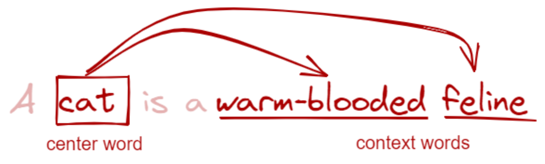
As John Rupert Firth, a famous linguist, once said: “You shall know a word by the company it keeps.”3 In this step, we create pairs consisting of each word in our vocabulary and its context (“the company it keeps”). We call the former as the center word and the latter as the context word.
clean_text function should’ve removed them at this point.You shall know a word by the company it keeps - John Rupert Firth
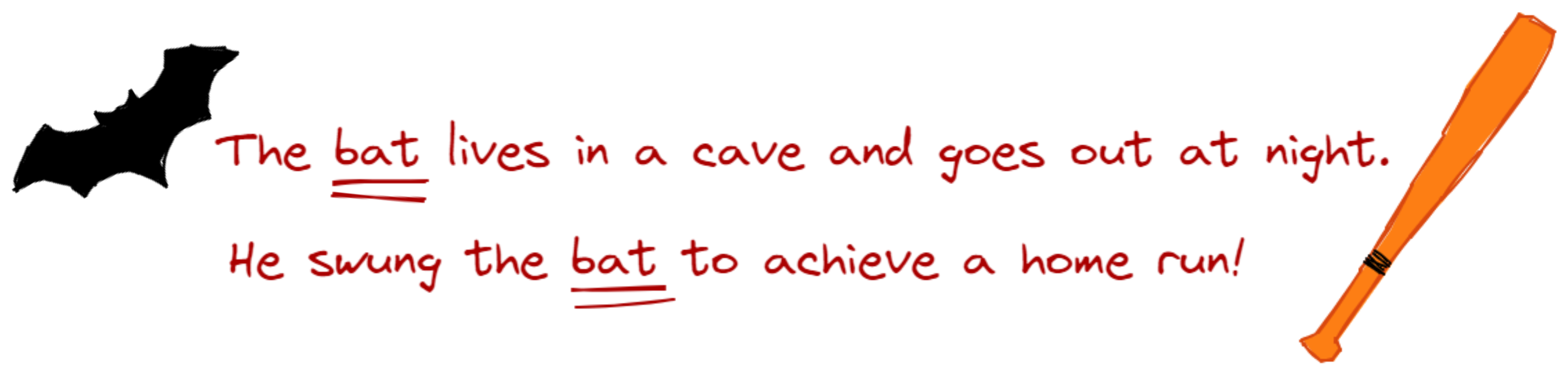
Context is important to understand meaning. Take the word bat for example. We don’t know what it means in isolation, but in a sentence, its meaning becomes crystal clear:
We can stretch this further: do you know the meaning of the words frumious, Jabberwock, and Jubjub? Well, we can only guess. But in the context of other words (in this case a poem), we can infer their meaning:
Beware the Jabberwock, my son!
The jaws that bite, the claws that catch!
Beware the Jubjub bird, and shun
The frumious Bandersnatch!
By looking at the context of each word, we now know that Jabberwock is a noun and can be something dangerous because of the word ‘beware.’ It also has ‘jaws’ and ‘claws’ that bite and catch. Frumious, on the hand, is an adjective that describes a Bandersnatch. Lastly, Jubjub could be a type of bird that one should be beware of. Well…truth is, these words were just made up! I lifted them from Lewis Carroll’s poem, “Jabberwocky”, in the novel Through the Looking-Glass. Awesome, huh?
We can also control the neighbors of a word through its window size. A size of 1 means that a center word only sees adjacent words as its neighbor. Too high a window and your context becomes less informative, too low and you fail to capture all of its nuance.
Too high a window and your context becomes less informative, too low and you fail to capture all of its nuance.
Now, we write a function to get word pairs from a sentence:
def create_word_pairs(
    text: List[str],
    window: int = 2
) -> List[Tuple[str, str]]:
    word_pairs = []
    for idx, word in enumerate(text):
        for w in range(window):
            if idx + 1 + w < len(text):
                pair = tuple([word] + [text[idx + 1 + w]])
                word_pairs.append(pair)
            if idx - w - 1 >= 0:
                pair = tuple([word] + [text[idx - w - 1]])
                word_pairs.append(pair)
    return word_pairs
Note that at this stage, we’ve already cleaned and tokenized our sentences. We now pass a string of tokens and obtain a list of pairs.
text = "A cat is a warm-blooded feline."
cleaned_tokens = clean_text(text)  # ["cat", "warm-blooded", "feline"]

# Get word pairs
create_word_pairs(cleaned_tokens)
From here we obtain six pairs:
[('cat', 'warmblooded'),
 ('cat', 'feline'),
 ('warmblooded', 'feline'),
 ('warmblooded', 'cat'),
 ('feline', 'warmblooded'),
 ('feline', 'cat')]
We do this step for each text in our corpus. In the end, we obtain a large list of pairs containing every word in our vocabulary and their corresponding neighbor. The larger the corpus, the larger the expressivity of our word pairs.
In a way, having these pairs allows us to see which words tend to stick together. Later on, we will train a model that can understand this affinity, i.e., given a word \(X\), what’s the probability that a word \(Y\) will show up? In the next section, we’ll jumpstart this stage by preparing our dataset.
3. Encode to one-hot vectors 🖥️
After obtaining word pairs, the next step is to convert them into some numerical format. We won’t be overthinking this too much, so we’ll treat those numbers similar to how we treat words— as discrete symbols. We accomplish this with one-hot encoding.
In one-hot encoding, we prepare a table where each word in our vocabulary is
represented by a column. Our word columns don’t have to be in a specific order,
although I prefer sorting them alphabetically. To encode a word, we simply write
1 in the column where it is located and write 0 elsewhere:
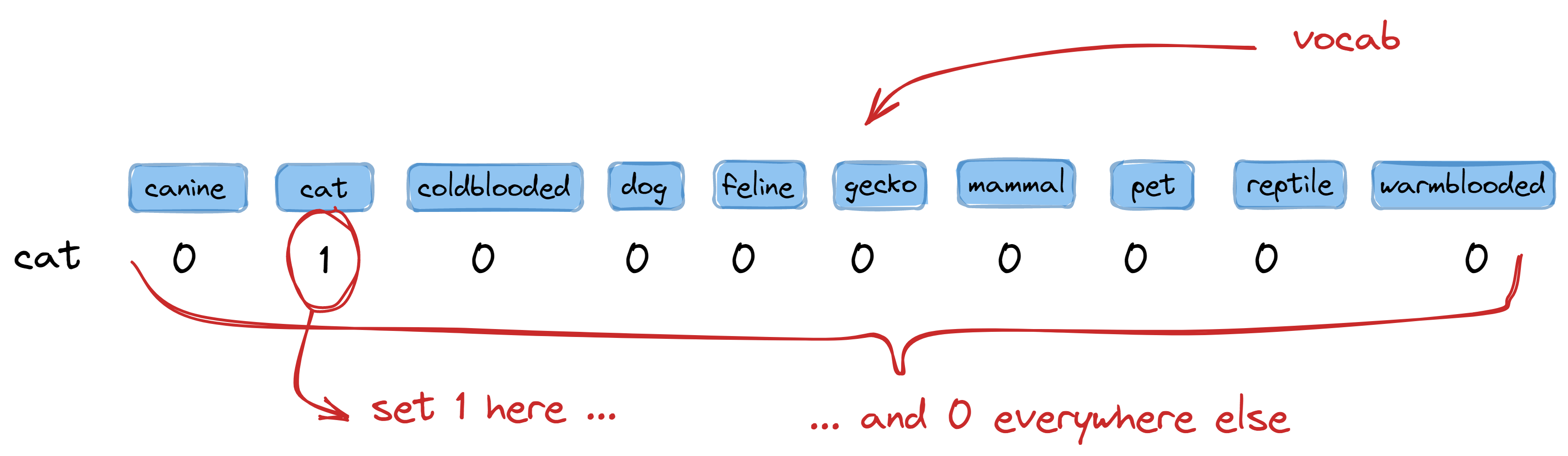
So for our corpus with a vocabulary size of 10, we create a table with ten columns.
To encode the word cat, we write 1 in the second column (where cat is located) and 0
elsewhere. This gives us the encoding:
>>> one_hot_encode("cat")  # I will show its implementation later!
[0, 1, 0, 0, 0, 0, 0, 0, 0, 0]
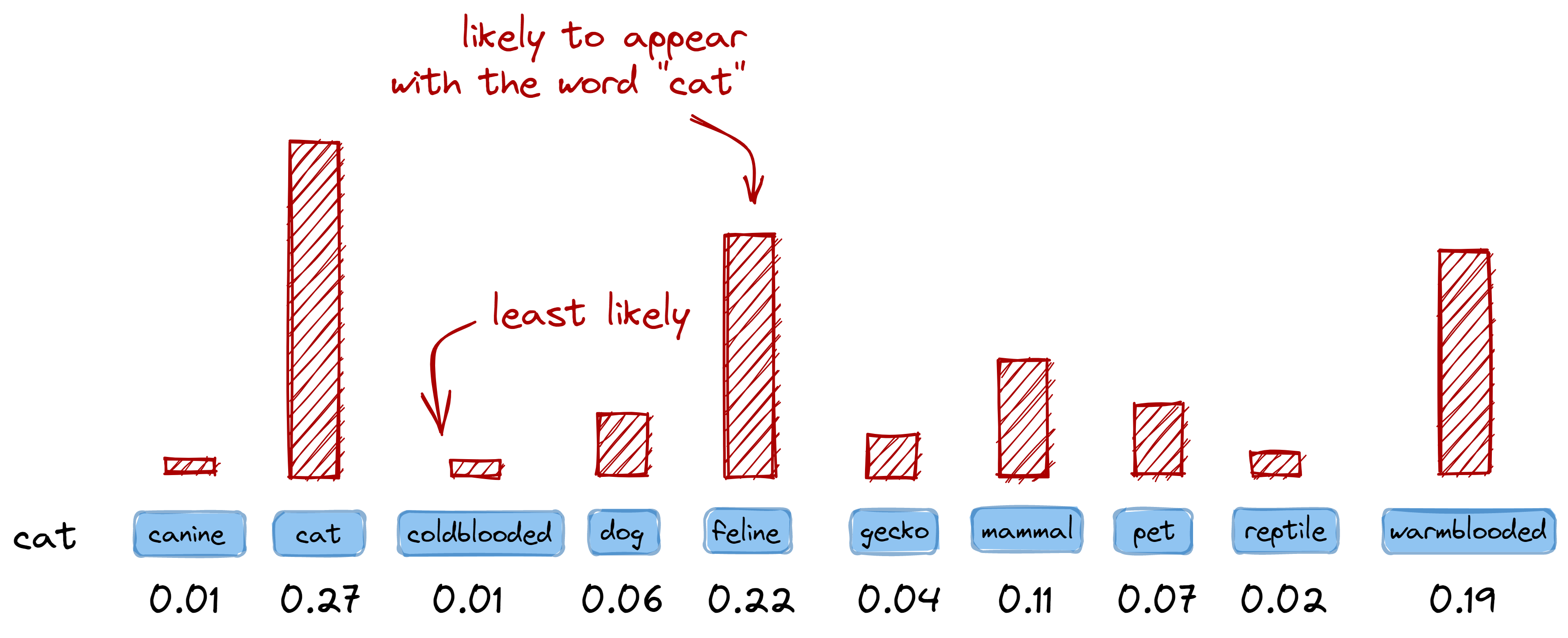
One advantage of one-hot encoding is that it allows us to interpret the encoded
vector as a probability distribution over our vocabulary. For example, if I have
a center word cat, we can then check how likely other words in our vocab will
appear as a context word:
# Note: not actual values. A highly-contrived example
# Numbers are just provided for illustration
>>> {v: l for v, l in vocab, get_likelihood("cat"))}
{
 "canine": 0.01,
 "cat": 0.27,
 "coldblooded": 0.01,
 "dog": 0.06,
 "feline": 0.22,
 "gecko": 0.04,
 "mammal": 0.11,
 "pet": 0.07,
 "reptile": 0.02,
 "warmblooded": 0.19,
}
One-hot encoding allows us to interpret the encoded vector as a probability distribution over our vocabulary.
This also means that if we have the following word pair ("cat", "feline"),
their encoding can be interpreted as: “the word feline is likely to appear
given that the word cat is present.” It is consistent as long as we think of
zeroes and ones as probabilities:
>>> one_hot_encode("cat")
[0, 1, 0, 0, 0, 0, 0, 0, 0, 0]
>>> one_hot_encode("feline")
[0, 0, 0, 0, 1, 0, 0, 0, 0, 0]
One advantage of one-hot encoding is that it allows us to interpret the encoded vector as a probability distribution over our vocabulary.
Now, let’s write a function to create one-hot encoded vectors from all our word pairs and vocabulary. The vocabulary will guide us on the placement and length of the one-hot vector. Lastly, instead of taking a single word, we’ll take a list of word pairs to make things easier later on:
from typing import List, Tuple

def one_hot_encode(
    pairs: List[Tuple[str, str]],
    vocab: List[str]
) -> Tuple[List, List]:

    # We'll sort the vocabulary first.
    # It's not required, but it makes bookkeeping easier
    n_words = len(sorted(vocab))

    ctr_vectors = []  # center word placeholder
    ctx_vectors = []  # context word placeholder

    for pair in pairs:

        # Get center and context words
        ctr, ctx= pair
        ctr_idx = vocab.index(ctr)
        ctx_idx = vocab.index(ctx)

        # One-hot encode center words
        ctr_vector = [0] * n_words
        ctr_vector[ctr_idx] = 1
        ctr_vectors.append(ctr_vector)

        # One-hot encode context words
        ctx_vector = [0] * n_words
        ctx_vector[ctx_idx] = 1
        ctx_vectors.append(ctx_vector)

    return ctr_vectors, ctx_vectors
Now if we pass all our word pairs and vocabulary, we’ll get their corresponding one-hot encoded center and context vectors:
sample_word_pairs = [("cat", "feline"), ("dog", "warm-blooded")]
vocab = ["canine", "cat", "cold-blooded", ...]

center_vectors, context_vectors = one_hot_encoded(sample_word_pairs, vocab)
print(center_vectors)
# gives:
# [[0, 1, 0, 0, 0, 0, 0, 0, 0, 0],
#  [0, 0, 0, 1, 0, 0, 0, 0, 0, 0]]
# for "cat" and "dog", our center words
print(context_vectors)
# gives:
# [[0, 0, 0, 0, 1, 0, 0, 0, 0, 0],
#  [0, 0, 0, 0, 0, 0, 0, 0, 0, 1]]
# for "feline" and "warm-blooded", our context words
In the next section, we will be using these two sets of vectors to train a neural network model. The center vectors will act as our inputs, whereas the context vectors will act as our labels.
4. Train a model 🤖
Because we now have a collection of center words with their corresponding context words, it’s now possible to build a model that asks: “what is the likelihood that a context word \(y\) appears given a center word \(X\)?” or simply, \(P(y\vert x ; \theta)\).
To illustrate this idea: if the words warm-blooded, canine, and animal often appear alongside the word dog, then that means we can infer something informative about dogs. We just need to know how likely these words will come up, and that will be the role of our model.
To train a model, we will use the center words as our input, and the context words as our labels. We will build a neural network of size 10-2-10 with a softmax layer in its output:
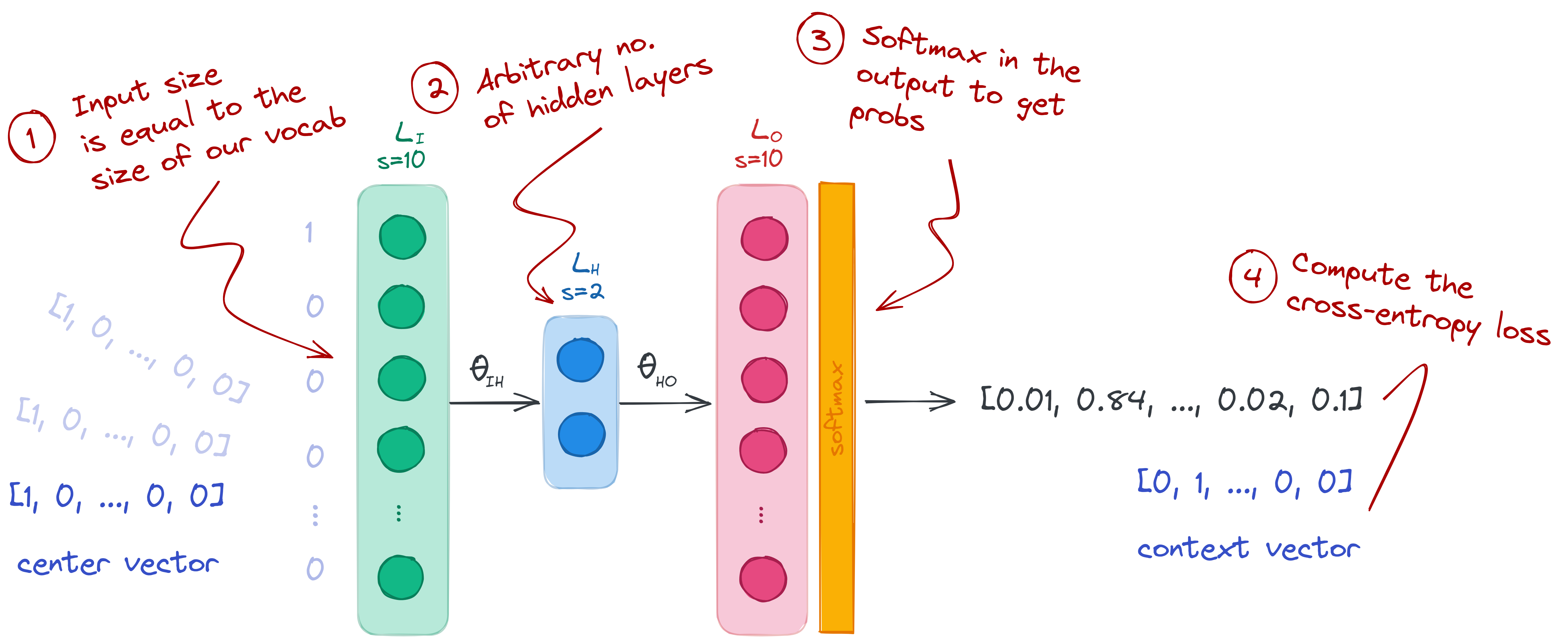
- Input layer (size 10): we set our input layer to the size of our vocabulary. We don’t need to add an activation layer, so we just leave it as it is.
- Hidden layer (size 2): this can be any arbitrary size, but I set it to 2 so that I can plot the weights in a graph. It’s also possible to set a higher number, and perform Principal Component Analysis (PCA) later on.
- Output layer (size 10 with softmax): we set the number of nodes to 10 so that we can compare it with the context vectors. The softmax activation is important so that we can treat the output as probabilities and use cross-entropy loss. To learn more about softmax, check my post on the negative log-likelihood.
Now, let’s construct our neural network. We’ll use the following third-party modules:
import torch
import torch.optim as optim
from torch import nn
We build our network based on the size of our center and context vectors. For the hidden layer, we set an arbitrary size of 2.
# Prepare layer sizes
input_dim = len(center_vectors[0])
hidden_dim = 2
output_dim = len(context_vectors[0])

# Build the model
model = nn.Sequential(
    nn.Linear(input_dim, hidden_dim),
    nn.Linear(hidden_dim, output_dim),
)
Next we prepare our loss function and optimizer. We will use cross-entropy loss
to compute the difference between the model’s output and the context vector. In
Pytorch, softmax is already included when using the
torch.nn.CrossEntropyLoss
class, so there’s no need to add it in our model definition:
# In Pytorch, Softmax is already added when using CrossEntropyLoss
loss_fn = torch.nn.CrossEntropyLoss()
optimizer = optim.Adam(model.parameters(), lr=1e-4)
We also convert our vectors into Pytorch’s
FloatTensor data type. At this
stage, I’ll also call the center and context vectors as X and y
respectively, just to be consistent with common machine learning naming schemes:
X = torch.FloatTensor(center_vectors)
y = torch.FloatTensor(context_vector)
Lastly, we write our training loop. Because we’re using a deep learning
framework, we don’t have to write the backpropagation step by hand. Instead, we
simply call the backward()
method
from the loss function:
for t in range(int(1e3)):
    # Compute forward pass and print loss
    y_pred = model(X)
    loss = loss_fn(y_pred, torch.argmax(y, dim=1))
    # Zero the gradients before running the backward pass
    optimizer.zero_grad()
    # Backpropagation
    loss.backward()
    # Update weights using gradient descent
    optimizer.step()
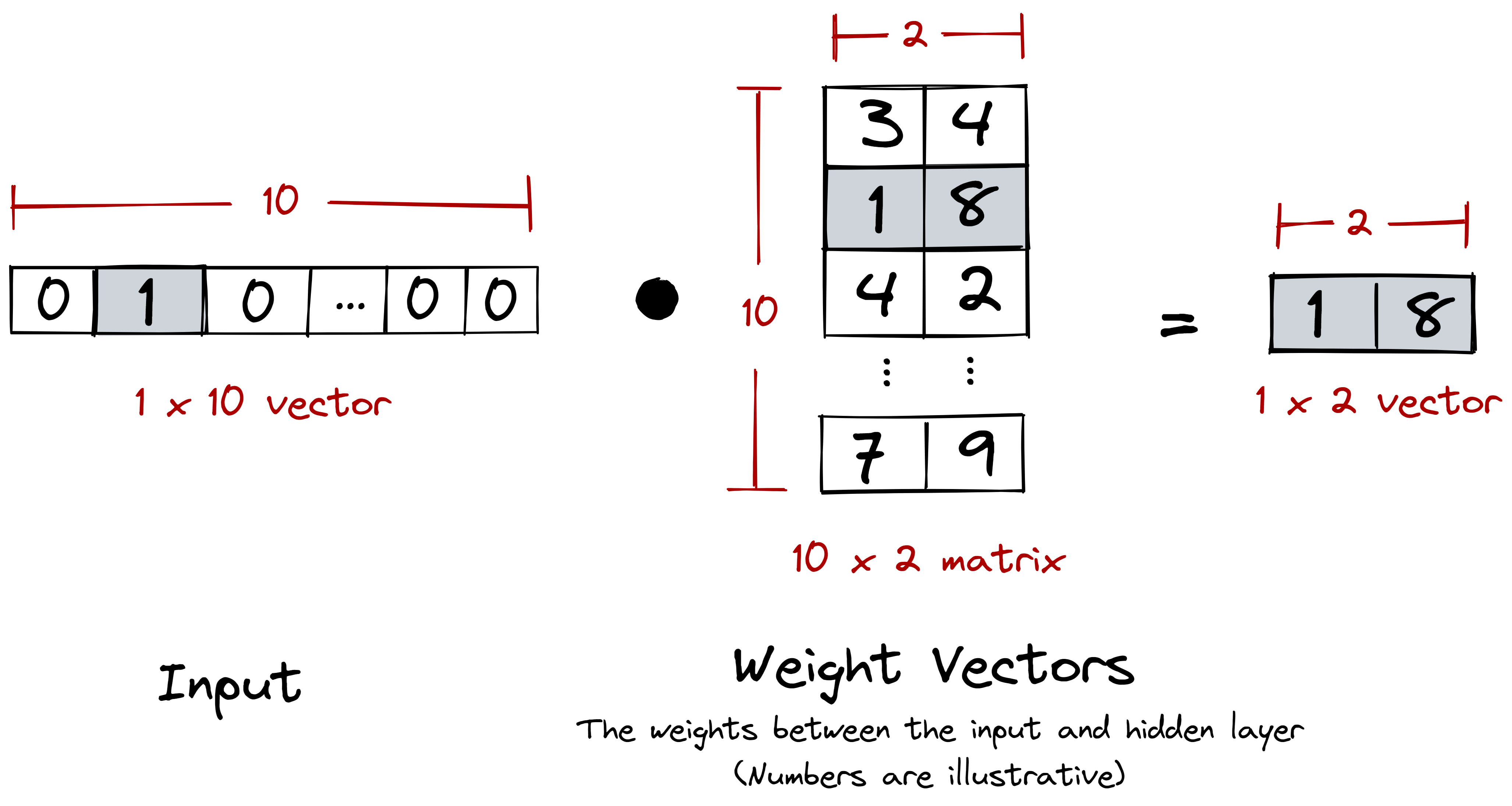
After training the model, we can now access its weights. We’ll obtain, in particular, the weights between the input and hidden layers:
name, weights = list(model.named_parameters())[0]
w = weights.data.tolist()
These weights are, in fact, our word vectors— congratulations! They are of the same size as our hidden layer. I’ve set their dimension to 2 so that we can plot the vectors right away into a graph. In the next section, we’ll show what this graph looks like to get a deeper look into the behaviour of our word vectors.
5. Post: on word vectors 🧮
After training our model, we took the weights between the input and hidden layers to obtain our word embeddings. We specifically chose these weights because they act as a lookup table for translating our one-hot encoded vectors into a more suitable dimension.
The intermediary weight matrix (weights between the input and hidden layers) acts as a lookup table that translates one-hot encoded vectors into a different dimension.
And this is definitely what we want. One-hot encoded vectors are sparse and
orthogonal: there’s really nothing that informative between [0 0 ... 1 0]
and [1 0 ... 0 0]. Instead, we want a dense vector where we can draw
meaningful semantic relations from. Our weight matrix performs this
transformation for us.
By having these dense and continuous relationships, we can even represent them into a graph!
Notice how semantically related words are nearer to each other. For example, the words gecko, reptile, and cold-blooded were clustered together. The same goes for cat, dog, and warm-blooded. Even more so, these clusters of “lizards” and “mammals” are further far apart!
We didn’t encode these relationships, it was all due to how the model interpreted the words from our corpus. Sure, we wrote these sentences ourselves, but in practice we just have to scrape them from somewhere.
Conclusion
In this blogpost, we looked into the idea of generating our own word vectors from scratch. We achieved this by combining (1) a text corpus and (2) an encoding mechanism. The word vectors we generated are crude, but we learned a few things on how they came about. Truth is, what we just did is similar to the original skip-gram implementation of Word2Vec (Mikolov, et al, 2013): given a text corpus, we generate word pairs and train a neural network across them.
In production, it is more ideal to use ready-made word embeddings—they are more robust and generalizable. Of course, real-world NLP still requires finetuning, but using these vectors should already give you a headstart.
Lastly, I hope that this exercise made us more aware of how a text corpus can be a source of bias: a corpus made up of Reddit comments will produce an entirely different model compared to a corpus lifted from an encyclopedia. We can use this for better or for worse: we can train “domain-specific” language models to min/max our task, or release models in the wild that are inherently biased. Real-world NLP isn’t as easy as figuring out cats and dogs.
-
Corpus literally means body, as in “a body of text.” Also, its plural form is corpora, not “corpi.” Fun! ↩
-
Writing tip: I use stopwords to gauge how clear my writing is. Sometimes, when I use a lot of stopwords my writing becomes full of fluff. ↩
-
This quote by Firth in the 1950s is one of the foundational ideas of distributional semantics and modern statistical NLP as a whole! ↩