The Illustrated VQGAN
Text-to-image synthesis has taken ML Twitter by storm. Everyday, we see new AI-generated artworks being shared across our feeds. All of these were made possible thanks to the VQGAN-CLIP Colab Notebook of @advadnoun and @RiversHaveWings. They were able to combine the generative capabilities of VQGAN (Esser et al, 2021) and discriminative ability of CLIP (Radford et al, 2021) to produce the wonderful images we see today:
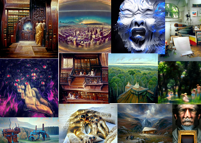
Figure: A few images generated by VQGAN-CLIP. Featuring works by
@advadnoun,
@RiversHaveWings, and Ryan
Moulton.
Also includes some works from @images_ai.
First things first: VQGAN stands for Vector Quantized Generative Adversarial Network, while CLIP stands for Contrastive Image-Language Pretraining. Whenever we say VQGAN-CLIP1, we refer to the interaction between these two networks. They’re separate models that work in tandem.
In essence, the way they work is that VQGAN generates the images, while CLIP judges how well an image matches our text prompt. This interaction guides our generator to produce more accurate images:

Figure: The VQGAN model generates images while CLIP guides the process. This is
done throughout many iterations until the generator learns to produce more
“accurate” images.
However, I’m more interested in how VQGAN works. It seems to prescribe a theory of perception that I find interesting. That’s why I’ll be focusing on the paper, “Taming Transformers for high-resolution images synthesis.” On the other hand, if you wish to learn more about CLIP, I suggest reading OpenAI’s explainer—it’s comprehensive and accessible.
Contents
Our discussion will follow a bottom-up approach, i.e., we’ll start with how we perceive images, then build the system from the ground up. In the end, our goal is to understand how each part of VQGAN’s architecture works and why they were chosen to perform that task.
Ready? Let’s go!
How we see images: a theory of perception
One thing that I like about VQGAN is that it prescribes an explanation of how we see things— a theory of perception, if you may. As a motivating example, if I ask you to describe this picture below, what would you say?
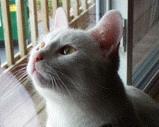
Figure: If I ask you to describe this picture, what would you say?
Some of you may describe this as “a white cat looking up,”
or “a cat.” Nevertheless, we
seem to encounter images through discrete representations: cat, white
, or looking up. This theory of perception suggests that our visual
reasoning is symbolic, we ascribe meaning through discrete representations and
modalities.
This theory of perception suggests that our visual reasoning is symbolic, we ascribe meaning through discrete representations and modalities.
This symbolic approach allows us to understand relationships between different
words or symbols. In machine learning, this is commonly known as being able to
model long-range
dependencies. For
example, in the sentence “a white cat looking up,” we knew
that looking up refers to the cat’s action while white refers to
the cat’s description.
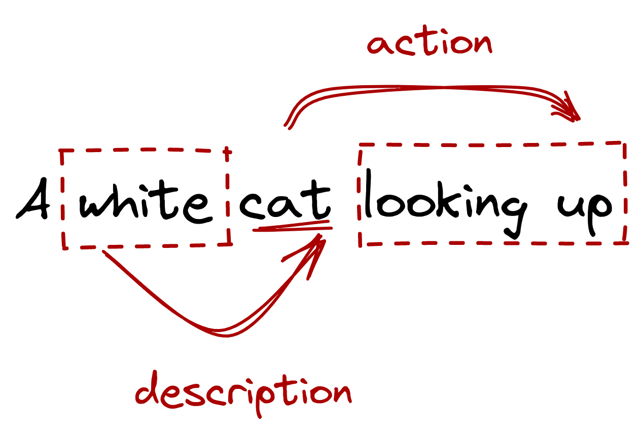
Figure: A discrete representation allows us to understand
relationships across symbols
or model long-range dependencies
Even though a lot of work has been done to explore complex reasoning through discrete representations (Salakhutdinov and Hinton, 2009, Mnih and Gregor, 2014, and Oord et al, 2017), most computer vision (CV) techniques don’t think in terms of modalities. Instead, they think in terms of pixels:
![]()
Figure: A close-up of the cat image. Each square represents a pixel with
three channels: red, green, and blue. Each channel has a continuous value and
affects the resulting color of the pixel.
Instead of thinking in terms of large chunks of information, common CV techniques focus on an image’s smallest unit. Each pixel channel—red, green, blue—represents a color value in a continuous scale. Needless to say, this may not be how our perception works.2
Despite all of these, we still shouldn’t ignore pixel-based approaches. Convolutional neural networks (CNN) proved that we can model local interactions between pixels by restricting interactions within their local neighborhood (i.e., the kernel). This allows us to “compose” pixels together and learn visual parts (Gu et al, 2018). The premier illustration for this is the feature map below, where a CNN learned how to compose pixels at varying layers of abstraction: pixels become edges, edges become shapes, and shapes become parts.
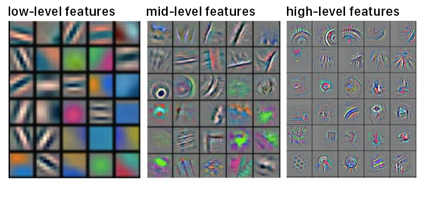
Figure: A convolutional neural network feature map showing features at
different levels
(photo from Tejpal Virdi, 2017)
Putting it all together, we now have two complementary techniques:
- an interesting view of perception that allows us to model long-range dependencies by representing images discretely; and—
- a pixel-based approach to learn local interactions and visual parts.
VQGAN was able to combine both of them. It can learn not only the (1) visual parts of an image, but also the (2) relationship (read: long-range dependencies) between these parts. We knew that the former can be done by a convolutional neural network, but we still have to discuss the latter. The table below summarizes the two:
| Approach | Examples | Can model | Analogy3 |
|---|---|---|---|
| Discrete | Sequence of symbols, words, phrases, and sentences | Long-range dependencies | Perceiving |
| Continuous4 | RGB channels in a pixel, convolutional filters, etc. | Local interactions and visual parts | Sensing |
VQGAN can learn not only the visual parts of an image, but also their relationships
In the next section, we’ll talk about how a Transformer (Vaswani et al, 2017) can model long-range dependencies between symbols. Transformers have been ubiquitous in natural-language processing, and seems to be a nice fit for modelling our theory of perception. However, it has one weakness: it doesn’t scale well to images.
Using Transformers to model interactions
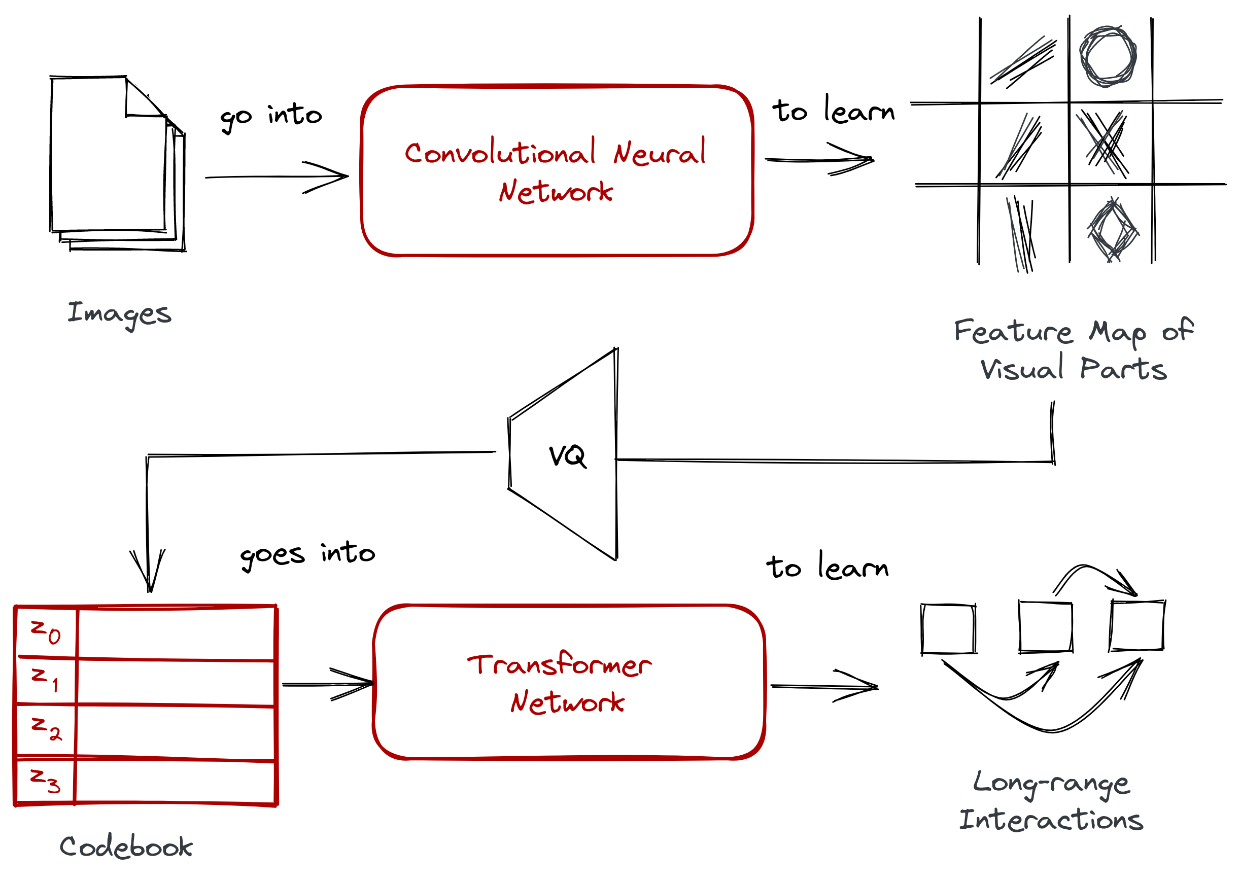
In the previous section, we introduced two approaches for handling images: (1) a continuous approach that learns visual parts using a convolutional neural network—
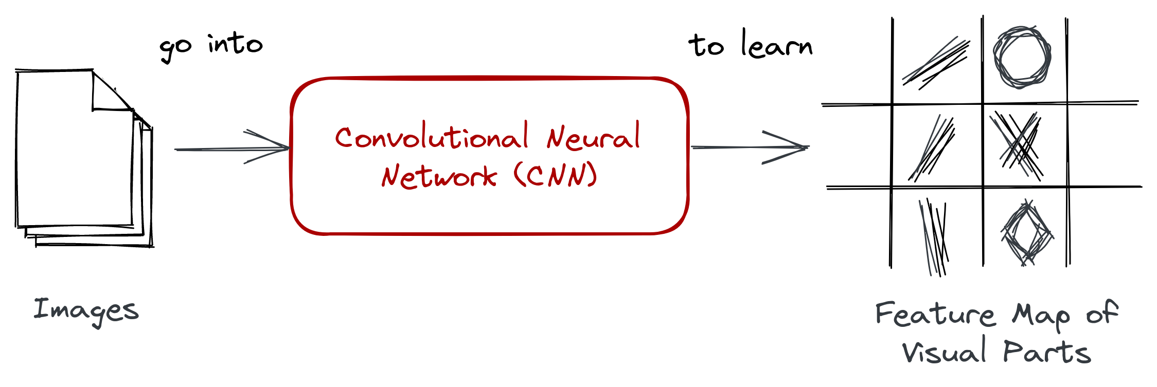
Figure: Given an image dataset, a convolutional neural network can learn
high-level features that we refer to as visual parts.
and (2) a discrete approach that learns long-range dependencies across them. We’ve also alluded that the latter is done by a Transformer network. Finally, we mentioned that VQGAN was able to take advantage of the two approaches.
The logical next step is to combine them together. One way is to directly feed the feature map into a Transformer. We can flatten the pixels of an image into a sequence and use that as input:
![]()
Figure: We can flatten the learned visual parts into a sequence and feed
it into a Transformer network (Note that the 4x4 size in the figure is illustrative).
Chen et al (2020) explored this approach. However, they encountered a limitation in the transformer network: its computation scales quadratically with the length of the input sequence. A 224 x 224 px image will have a length of \(224^2 \times 3\), way above the capacity of a GPU. As a result, they reduced the context by downsampling the 224-px image to 32-, 48-, and 64 pixel dimensions.
The reason Transformers scale quadratically is because of its attention mechanism (Vaswani et al, 2017): it computes for the pairwise inner product between each pair of the tokens. Through this method, it can learn about the long-range dependencies between tokens.
![]()
Figure: Transfromer works through its attention mechanism. It’s a
quadratic operation that scales with the length of the input sequence
There have been many attempts to circumvent the scaling issue, but at the cost of not being able to synthesize high-resolution imagery or making assumptions on pixel information. These were done by restricting the receptive fields of the attention modules (Parmar et al, 2018 and Weiseenborn et al, 2019), using sparse networks (Child et al, 2019), or training from image patches (Dosovitskiy et al, 2020). Nevertheless, we see a two-stage approach common across all works.
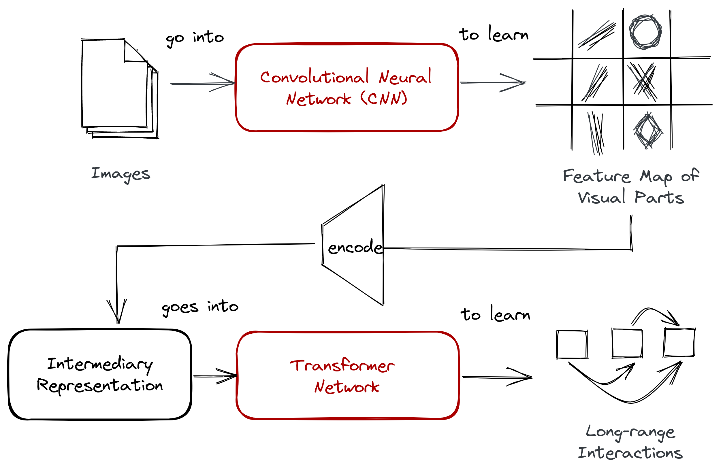
Figure: Common to most techniques is a two-stage approach that first learns
a representation from the image and encodes it to an intermediary form before
feeding into a transformer (or any autoregressive network).
VQGAN employs the same two-stage structure by learning an intermediary representation before feeding it to a transformer. However, instead of downsampling the image, VQGAN uses a codebook to represent visual parts. The authors did not model the image from a pixel-level directly, but instead from the codewords of the learned codebook.
VQGAN did not model the image from a pixel-level directly, but instead from the codewords of the learned codebook.
This codebook is created by performing vector quantization (VQ), and we’ll discuss more of it in the next section.
Expressing images through a codebook
In the previous section, we mentioned that VQGAN was able to solve Transformer’s scaling problem by using an intermediate representation known as a codebook. This codebook serves as the bridge for the two-stage approach found in most image transformer techniques:
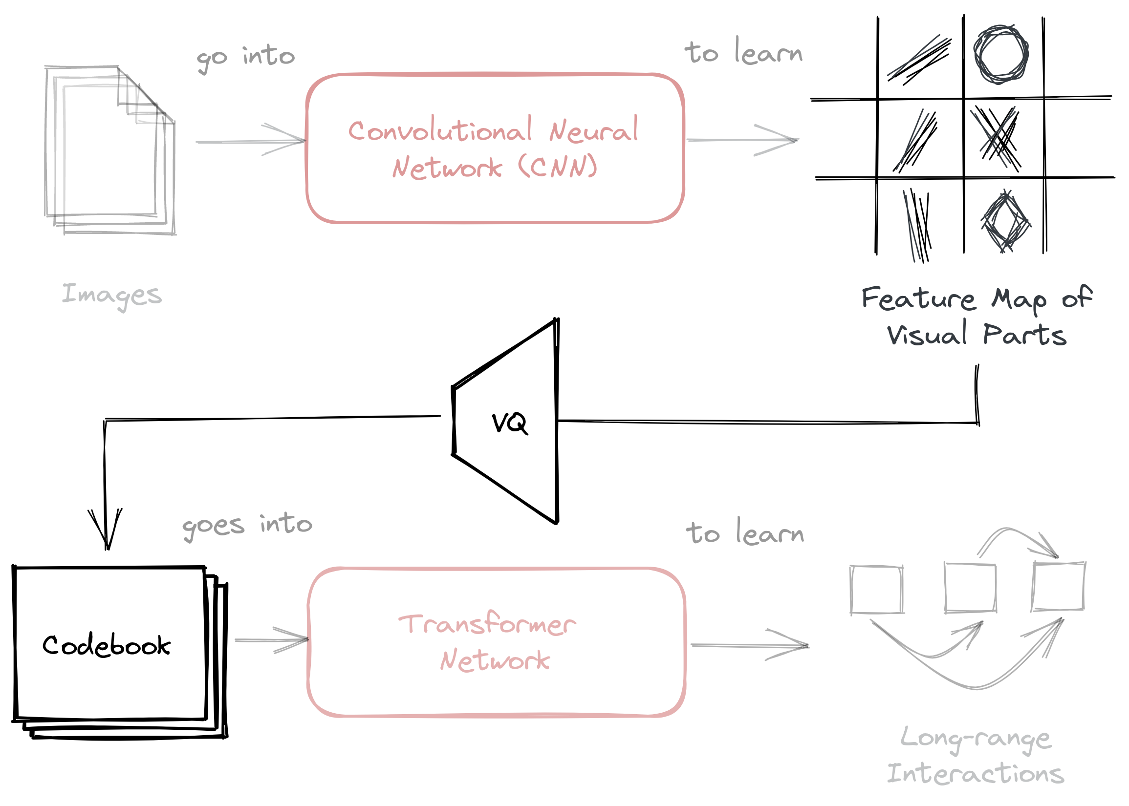
Figure: VQGAN employs a codebook as an intermediary representation before
feeding it to a transformer network. The codebook is then learned using vector
quantization (VQ).
The codebook is generated through a process called vector quantization (VQ), i.e., the “VQ” part of “VQGAN.” Vector quantization is a signal processing technique for encoding vectors. It represents all visual parts found in the convolutional step in a quantized form, making it less computationally expensive once passed to a transformer network.
One can think of vector quantization as a process of dividing vectors into groups that have approximately the same number of points closest to them (Ballard, 1999). Each group is then represented by a centroid (codeword), usually obtained via k-means or any other clustering algorithm. In the end, one learns a dictionary of centroids (codebook) and their corresponding members.
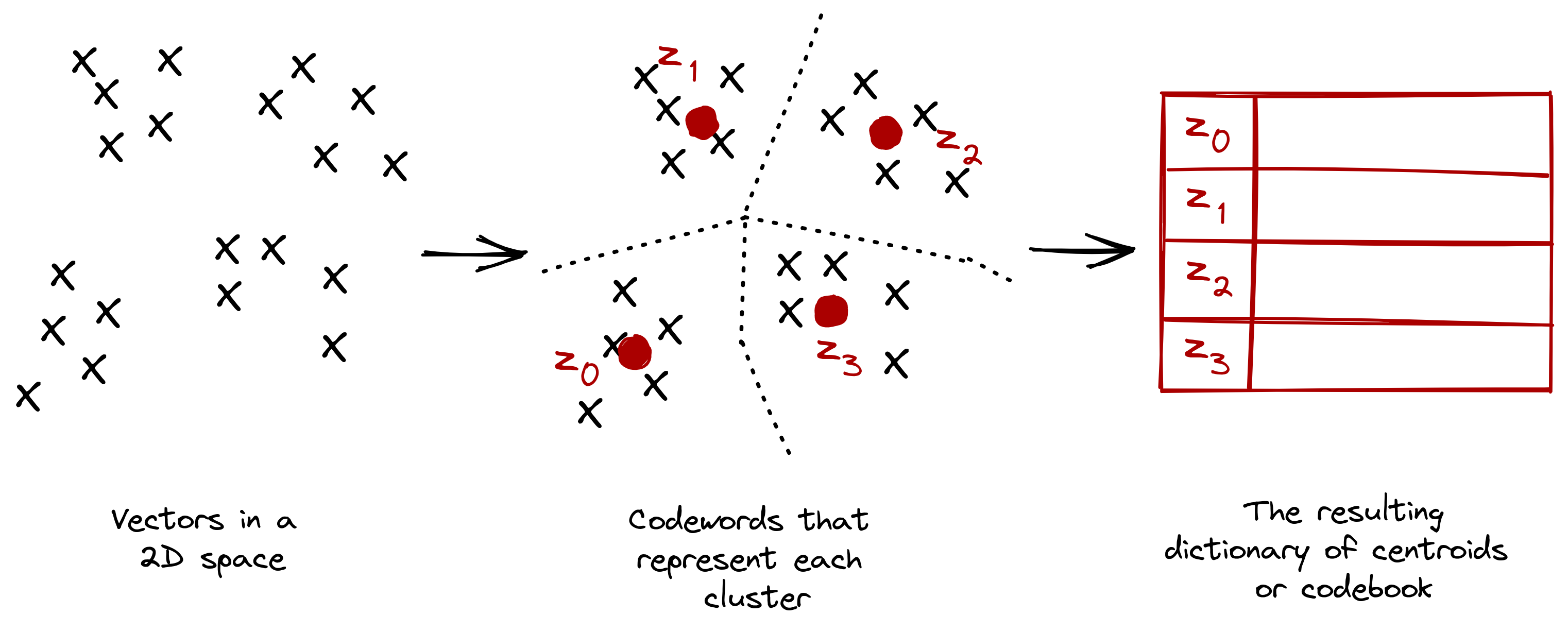
Figure: Vector quantization is a classic signal processing technique that
finds
the representative centroids for each cluster.
On a conceptual (and admittedly, handwavy) level, we can think of these
codewords as the discrete symbols that we used in our earlier examples: lady,
hat, night, moon, city, or rain. By training them with a transformer,
we start to uncover their relationships: “there’s moon at night,” “lady wears a
hat on her head,” or “it’s cloudy when it rains.”5
Now that we are familiar with the two-stage approach and the codebook, it’s time to put them all together and make a few adjustments to describe the system architecture of VQGAN.
Putting it all together
At this point, we now have all the ingredients needed to discuss VQGAN’s architecture:
- A convolutional neural network that takes a set of images to learn their visual parts. By taking advantage of a pixel’s local interactions, we can learn high-level features to construct new imagery.
- A transformer network that takes a sequence to learn their long-range interactions. Given a discrete representation, a transformer allows us to understand relationships across visual parts.
- A codebook obtained via vector quantization. It consists of discrete codewords that allows us to easily train a transformer on top of it.
However, we’ll make a few tiny adjustments:
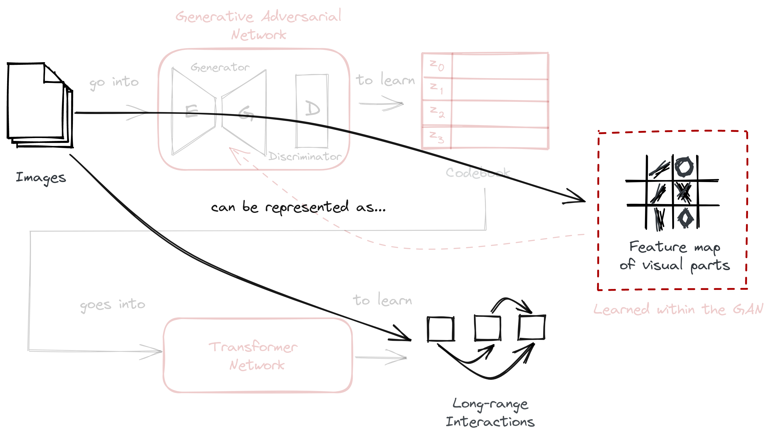
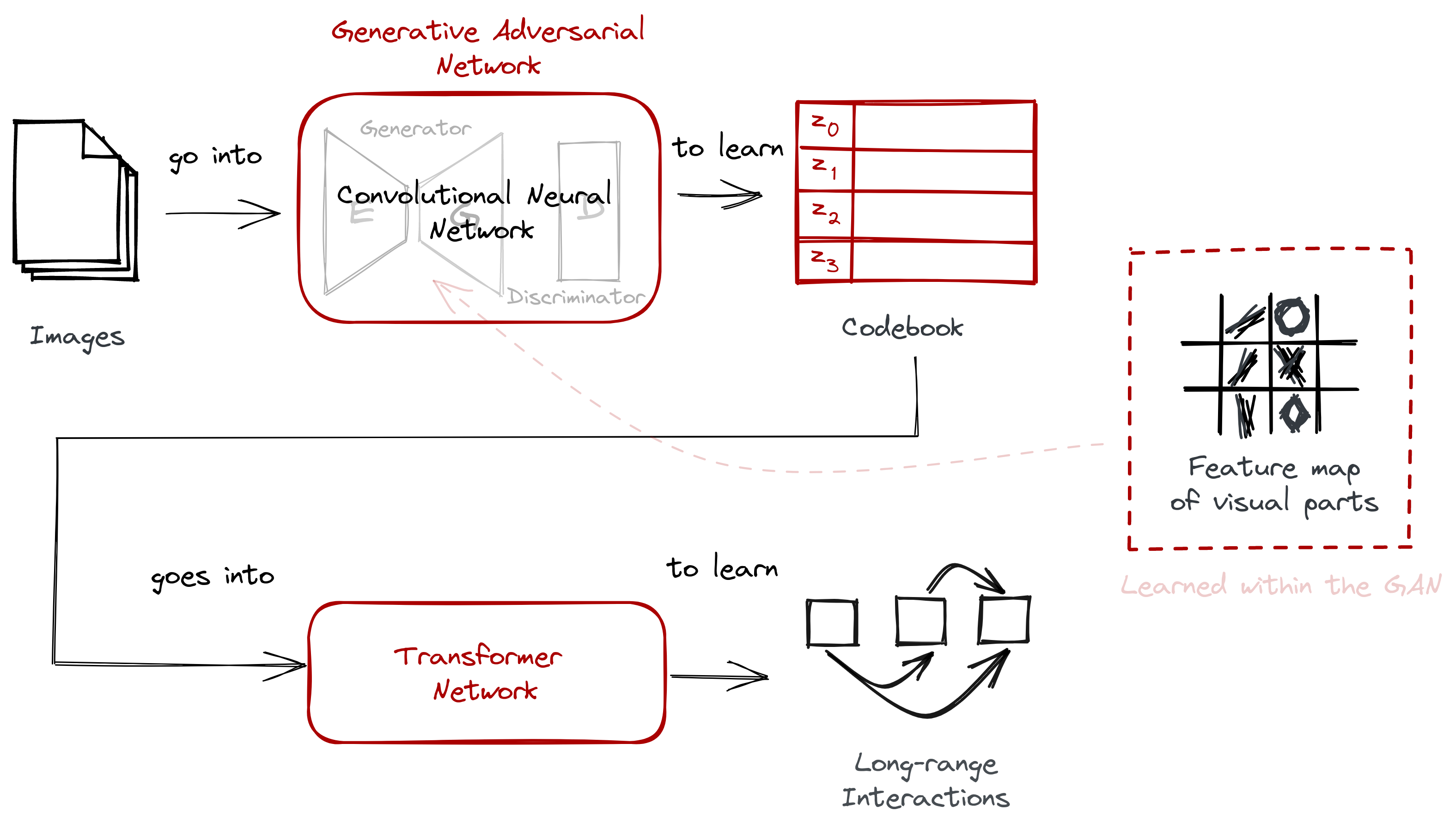
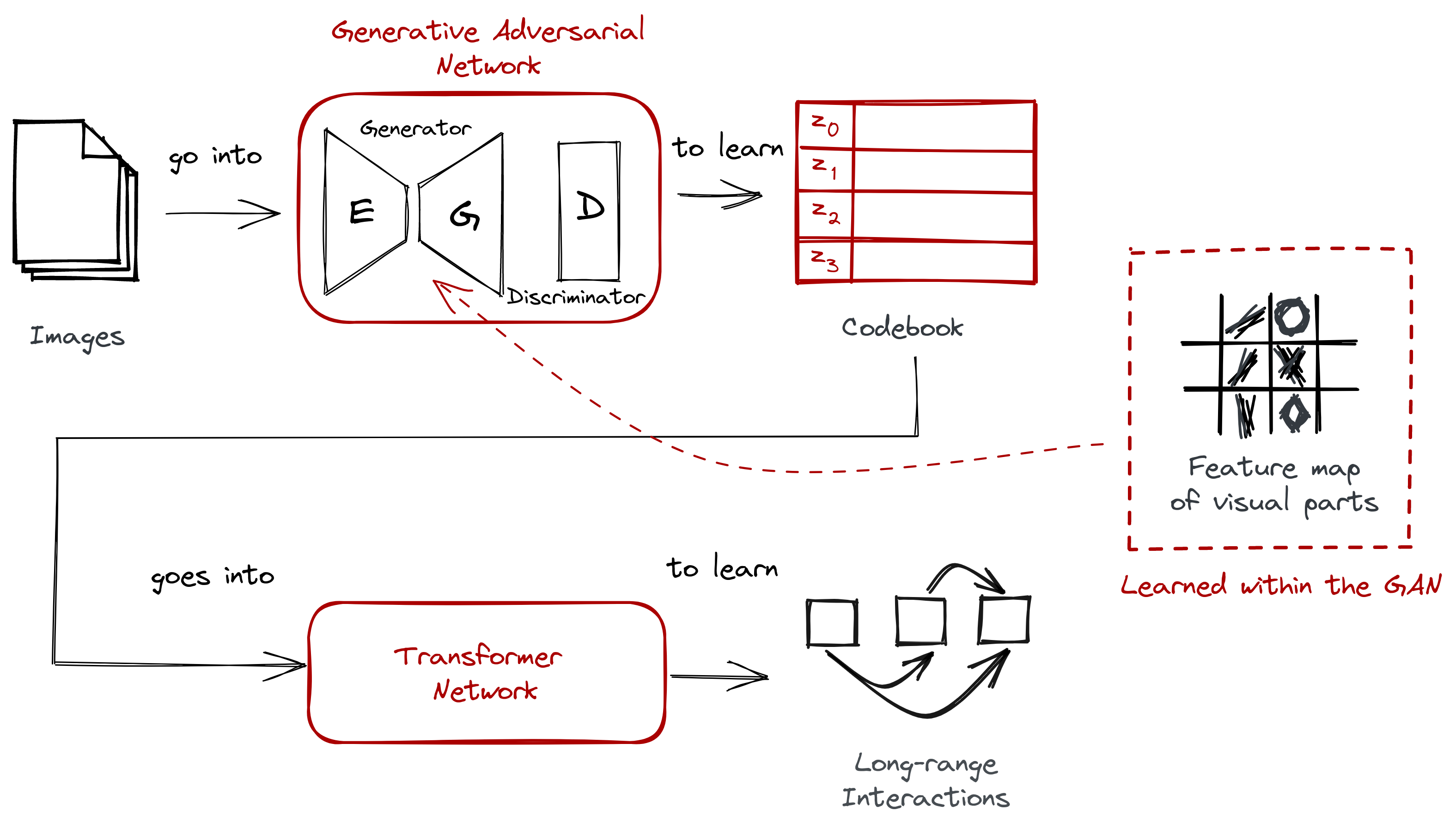
- We’ll replace the simple convolutional neural network with a generative adversarial network. The layers still perform a convolution operation, but with a GAN it synthesizes more distinct visual parts.
- Instead of having a separate process for vector quantization, VQGAN will learn the codebook right away. Learning the feature map of visual parts happens inside the GAN. It’s still the same two-stage approach
Below is the complete architecture diagram for VQGAN:
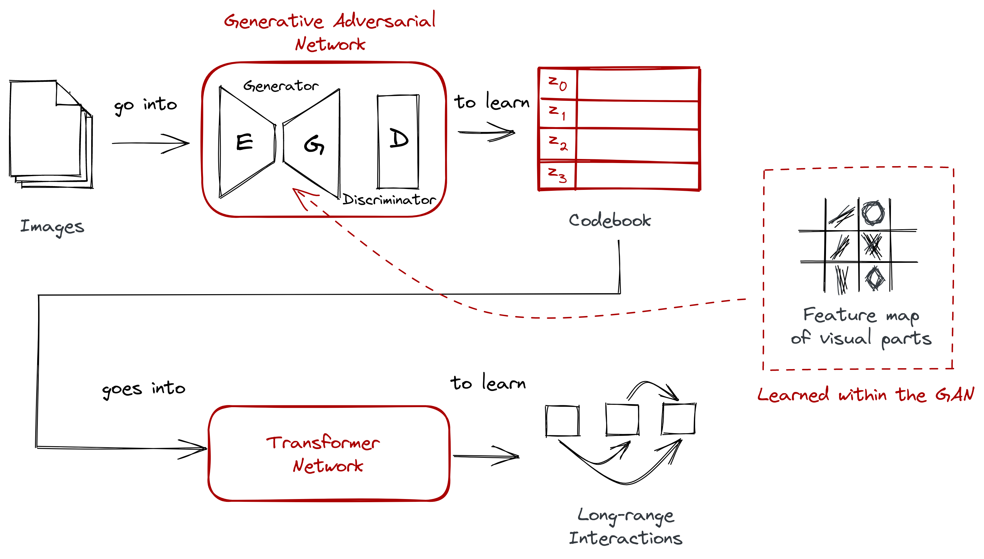
Figure: It’s still the two-stage approach, but with some minor changes: (1) instead of a typical CNN, we use a GAN, (2) instead of having a separate process for VQ, we learn the codebook right away.
In the next section, we’ll talk more about GANs and how the authors trained them to learn the codebook right away. In addition, we’ll also discuss sliding attention and how it affects Transformer training.
Training VQGAN
Due to its two-stage nature, training also happens in two major steps:
- Training the GAN from a dataset of images to learn not only its visual parts, but also their codeword representation, i.e., the codebook.
- Training the Transformer on top of the codebook with sliding attention to learn long-range interactions across visual parts.
Training the GAN
Earlier, we replaced the convolutional neural network with a generative adversarial network or a GAN (Goodfellow et al, 2014). Think of a GAN as an architecture composed of two competing neural networks:
- a generator \(N\) for creating new samples, and
- a discriminator \(D\) that classifies the samples as either real or fake.
The interaction between the two motivates the generator to fool the discriminator, enabling it to synthesize convincingly fake samples.
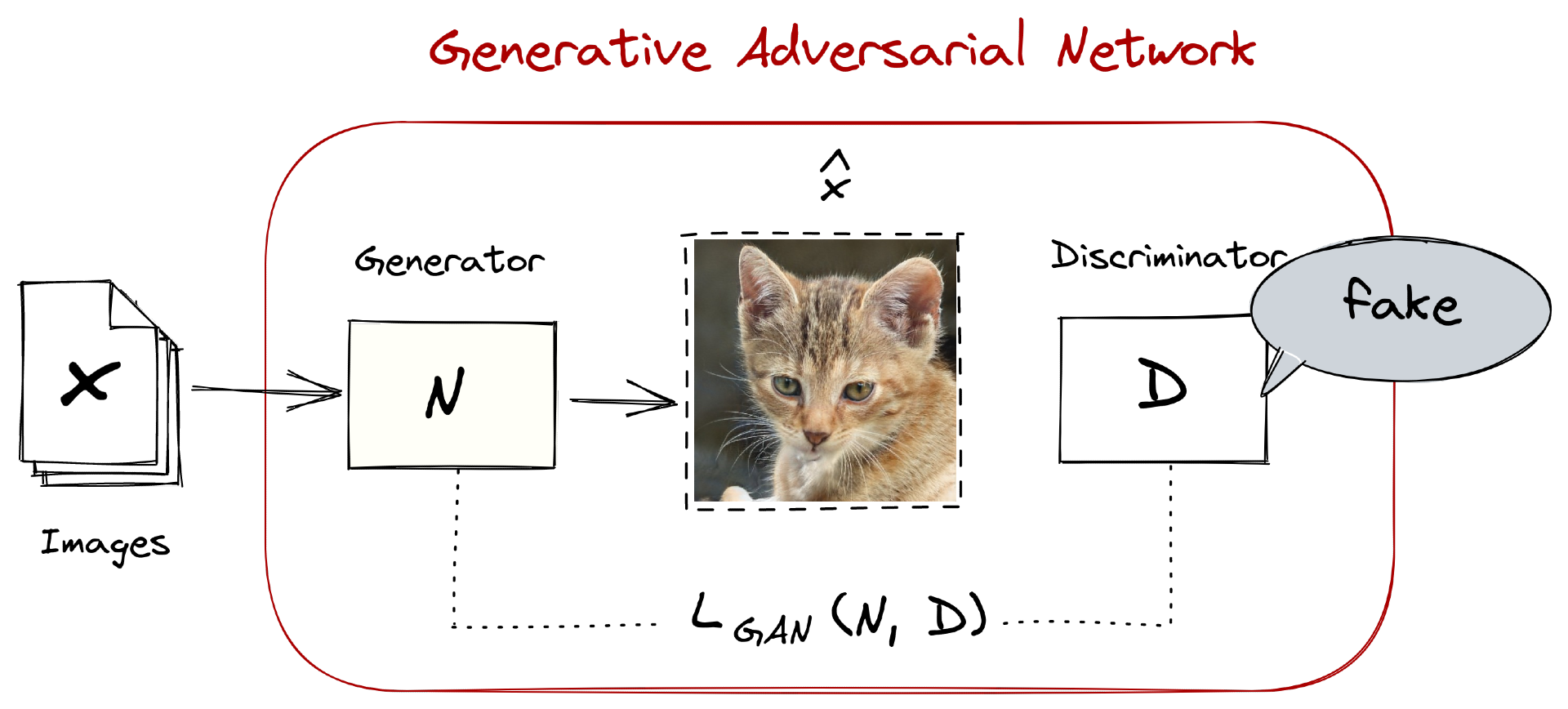
Figure: Illustration of a GAN. For simplicity, I drew the discriminator to
classify the whole image. In VQGAN, they employed a patch-based discriminator
(Isola et al, 2017),
where classification happens for each grid-like patch.
So if we have a real input \(x\) and a generated sample \(\hat{x}\), we evaluate our discriminator in its ability to differentiate between real and reconstructed images. We do so using the loss \(\mathcal{L}_{GAN}\):
\[\mathcal{L}_{GAN}(N,D) = [\log D(x) + log(1-D(\hat{x}))]\]In classic GAN literature, this is known as the minimax loss:
- The first term, \(\log D(x)\), measures the probability of the discriminator \(D\) to say that a real data instance \(x\) is actually real.
- The second term, \(\log(1-D(\hat{x}))\), measures the probability of the discriminator \(D\) to say that a generated instance \(\hat{x}\) is real.
If we look under the hood of VQGAN’s generator \(N\), we’ll see that it follows an encoder-decoder architecture. This setup is reminiscent of autoencoders, where the goal is to have a decoder \(G\) properly reconstruct the input \(x\). The theory is that if we have perfect reconstruction, then that means the encoder \(E\) has found a suitable representation of the data.
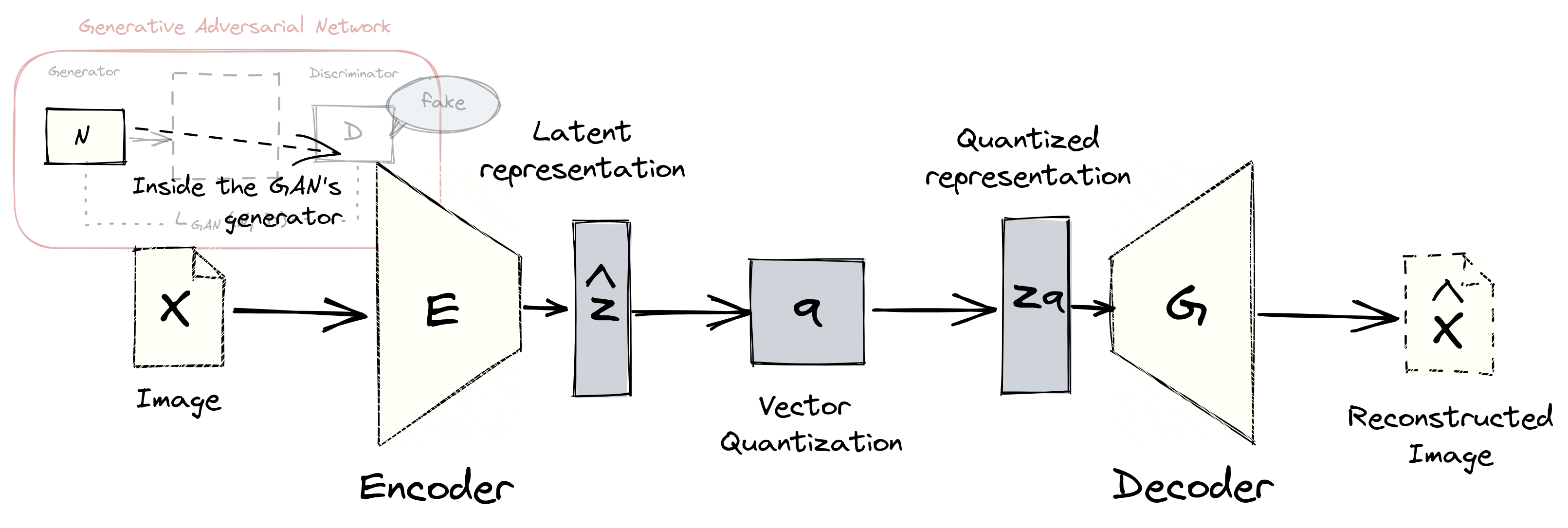
Figure: The GAN’s generator contains an autoencoder network. The
quantization step \(\mathbf{q}\) to produce the codebook \(Z\) is found between
the encoder \(E\) and decoder \(G\) networks.
Vector quantization also happens between the encoder and decoder networks. After encoding the input \(x\) into \(\hat{z}\), i.e., \(\hat{z} = E(x)\), we perform an element-wise operation \(\mathbf{q}\) to obtain a discrete version of the input:
\[z_{q} = \mathbf{q}(\hat{z}) := \text{arg min}_{z_k \in \mathcal{Z}} || \hat{z}_{ij} - z_k ||\]So instead of reconstructing from the encoder output \(\hat{z}\), we do it from its quantized form \(z_q\). Thus, the reconstructed image \(\hat{x} \approx x\) looks like this:
\[\hat{x} = G(z_\mathbf{q}) = G(\mathbf{q}(E(x)))\]The autoencoder model and the codebook were trained together using the loss function \(\mathcal{L}_{VQ}\):
\[\mathcal{L}_{VQ}(E, G, Z) = ||x-\hat{x}||^{2} + ||sg[E(x)] - z_\mathbf{q}||_2^2 + ||sg[z_\mathbf{q}] - E(x) ||_{2}^2\]It’s a bit hard to parse, so let’s take them one-by-one:
- The first term, \(||x-\hat{x}||^{2}\), is the reconstruction loss, it checks how well our network was able to approximate (via \(\hat{x}\)) our input \(x\) when given only its quantized version \(z_\mathbf{q}\). Note that this is computed as perceptual loss (Johnson and Li, 2016), not in a per-pixel basis.
- The second term, \(||sg[E(x)] - z_\mathbf{q}||_2^2\), optimizes our embeddings. The operation \(sg\) stands for “stop-gradient.” It is an identity function during forward pass, and has zero partial derivatives, thus constraining it to be constant.
- The last term,\(||sg[z_\mathbf{q}] - E(x) ||_{2}^2\), is called the commitment loss. It ensures that the encoder \(E\) commits to a particular representation of the image.
Finally, training VQGAN to obtain the optimal compression model \(Q^{\star}\) becomes a matter of combining the two losses from the autoencoder, \(\mathcal{L}_{VQ}\), and the GAN, \(\mathcal{L}_{GAN}\):
\[Q^{\star} = \text{arg min}_{E,G,Z} \text{max}_D \mathbb{E}_{x~p(x)} [\mathcal{L}_{VQ}(E, G, Z) + \lambda \mathcal{L}_{GAN}(N, D)]\]where \(Z\) is the codebook and \(\lambda\) is the adaptive weight.
When put together, we obtain the discrete capabilities of VQ, the rich expressivity of GANs, and the encoding capabilities of the autoencoder. This allows us to obtain richer and more distinct visual parts than a standard convolutional neural network.
Once we have learned the codebook \(Z\), then it is time to feed it into a transformer.
Training the transformer
Previously, we discussed how VQGAN trained the generative adversarial network. Training the first component of this two-stage system led us to learn the encoder \(E\), decoder \(G\), and codebook \(Z\). In this section, we’ll discuss how VQGAN trains the transformer.
We’re only interested with the codebook \(Z\) because it provides a discrete representation of our visual parts that can readily be fed to a transformer. To do so, we represent the images in terms of the codebook-indices of their embeddings. This means that the encoding \(z_{\mathbf{q}}\) of an image \(x\) can be represented as a sequence \(s\) from our codebook \(Z\), that is, \(s \in \{0, \dots, |Z| - 1\}\).
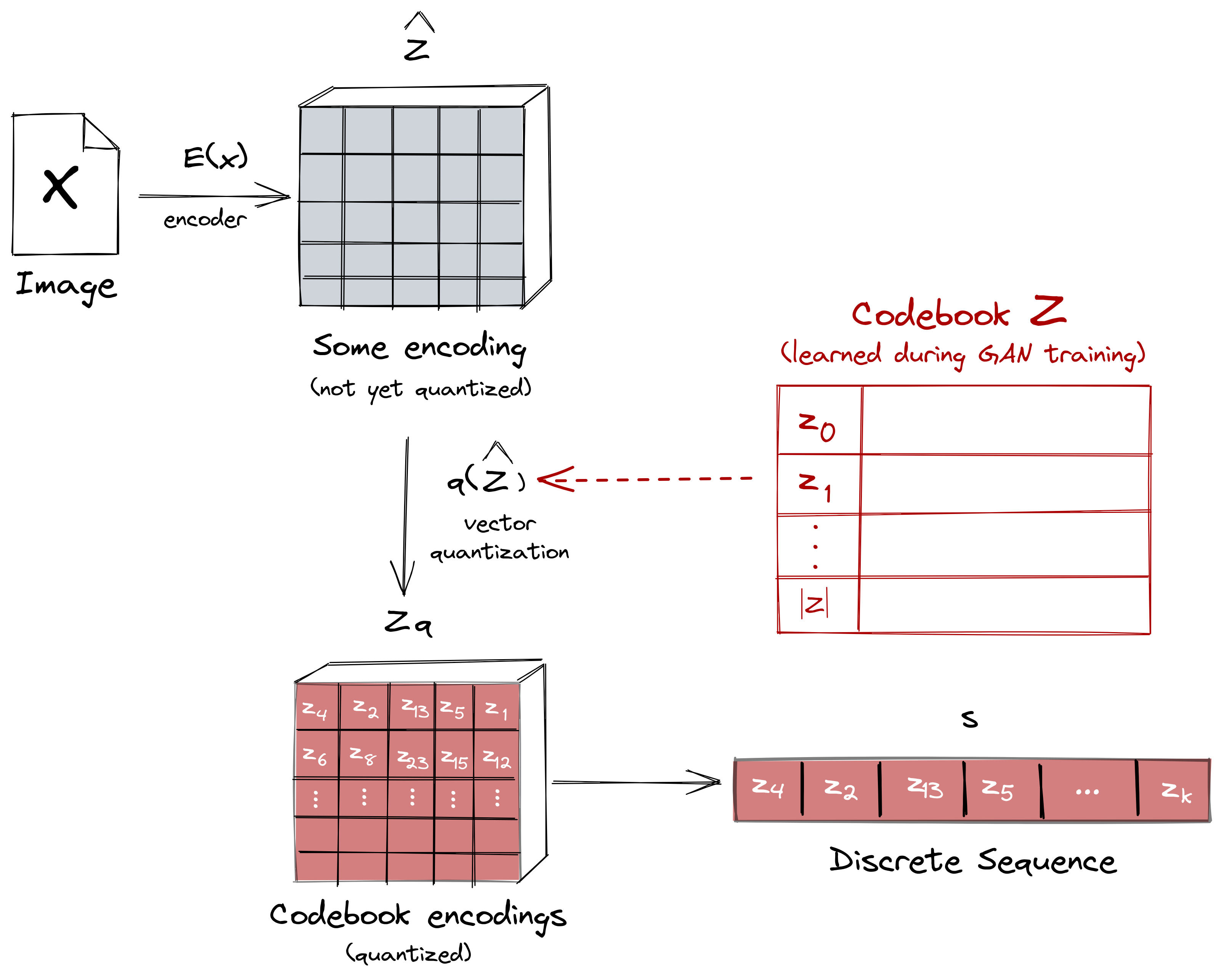
Figure: After training the first stage, we can now represent the images in
a sequence corresponding to the codebook-indices of their embeddings.
Now that we have our sequences, we can just train our transformer to predict the next index of an encoded sequence. So if we have indices \(s_{<i}\), the transformer predicts the distribution of possible next indices, \(p(s_i | s_{<i})\):
![]()
Figure: Training the transformer is done via next-word prediction similar to languages. If we wish to predict \(s_5\), we need to consider the symbols before that.
By doing so, we get to compute the likelihood as \(p(s) = \Pi_i p(s_i|s_{<i})\) and minimize the transformer loss \(\mathcal{L}_{\text{Transformer}} = \mathbb{E}_{x\sim p(x)} [-\log p(s)]\)— it’s more straightforward.
Lastly, when generating high-resolution images, the authors restricted the context via a sliding-window. This means that when generating each patch, it obtains information only from its neighbors. It’s a nice “trick” to improve resource-efficiency when using transformers.
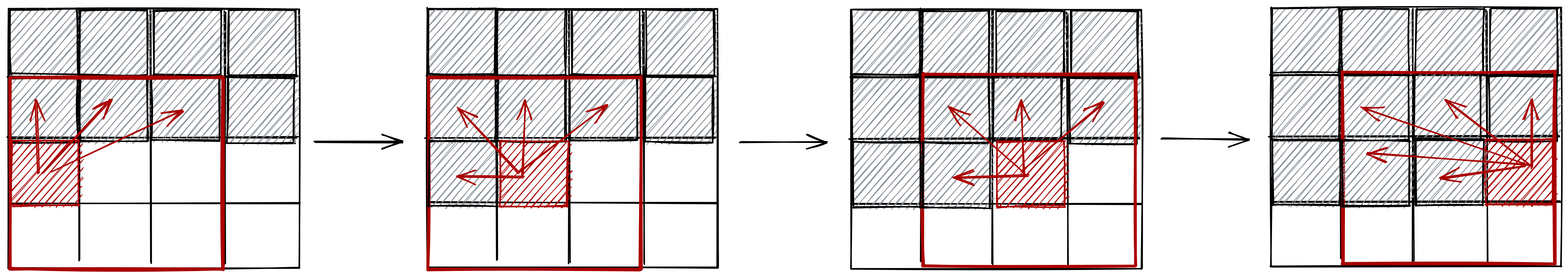
Figure: When sampling images, VQGAN used a sliding attention to different
patches so that sufficient context is still present.
Conclusion
In this blogpost, we looked into how VQGAN in VQGAN-CLIP works to generate and synthesize the high-resolution images we see today. The overall architecture looks like this:
First, we looked into the data itself, establishing a theory of perception where images can be describe through their discrete representations. This can be seen in contrast to usual computer vision techniques where pixels are the focus:
Then, we examined the two-stage approach implemented by VQGAN. It’s composed of a convolutional neural network in the form of a GAN, and a Transformer:

We also highlighted the difficulties in scaling the Transformer model, thus requiring the use of a codebook obtained via vector quantization. The codebook bridges the gap between the two stages.
Lastly, we discussed how the codebook was trained together with the two models. We started with training the GAN, then followed with training the Transformer. We learned that the GAN is composed of an encoder-decoder network as its generator, and that the Transformer uses a sliding-attention window when sampling images:
In the end, VQGAN was able to demonstrate how we can synthesize high-resolution imagery by taking advantage of both discrete and pixel-based representations of an image. This innovation has allowed us to create the wonderful artworks we see today. Moreover, it has spurred this new movement of “prompt engineering,” which allows us to define problems or domains into natural language tasks, and have a model guide us to a solution.
@article{miranda2021vqgan,
  title        = {The Illustrated VQGAN},
  author       = {Miranda, Lester James},
  journal      = {ljvmiranda921.github.io},
  url          = {\url{https://ljvmiranda921.github.io/notebook/2021/08/08/clip-vqgan/}},
  year         = {2021}
}
Appendix: Opinionated Tree of Knowledge
VQGAN takes a lot of inspiration from previous works in the field. Here’s my attempt to trace how each development led to the other until it coalesce to the VQGAN we know today.
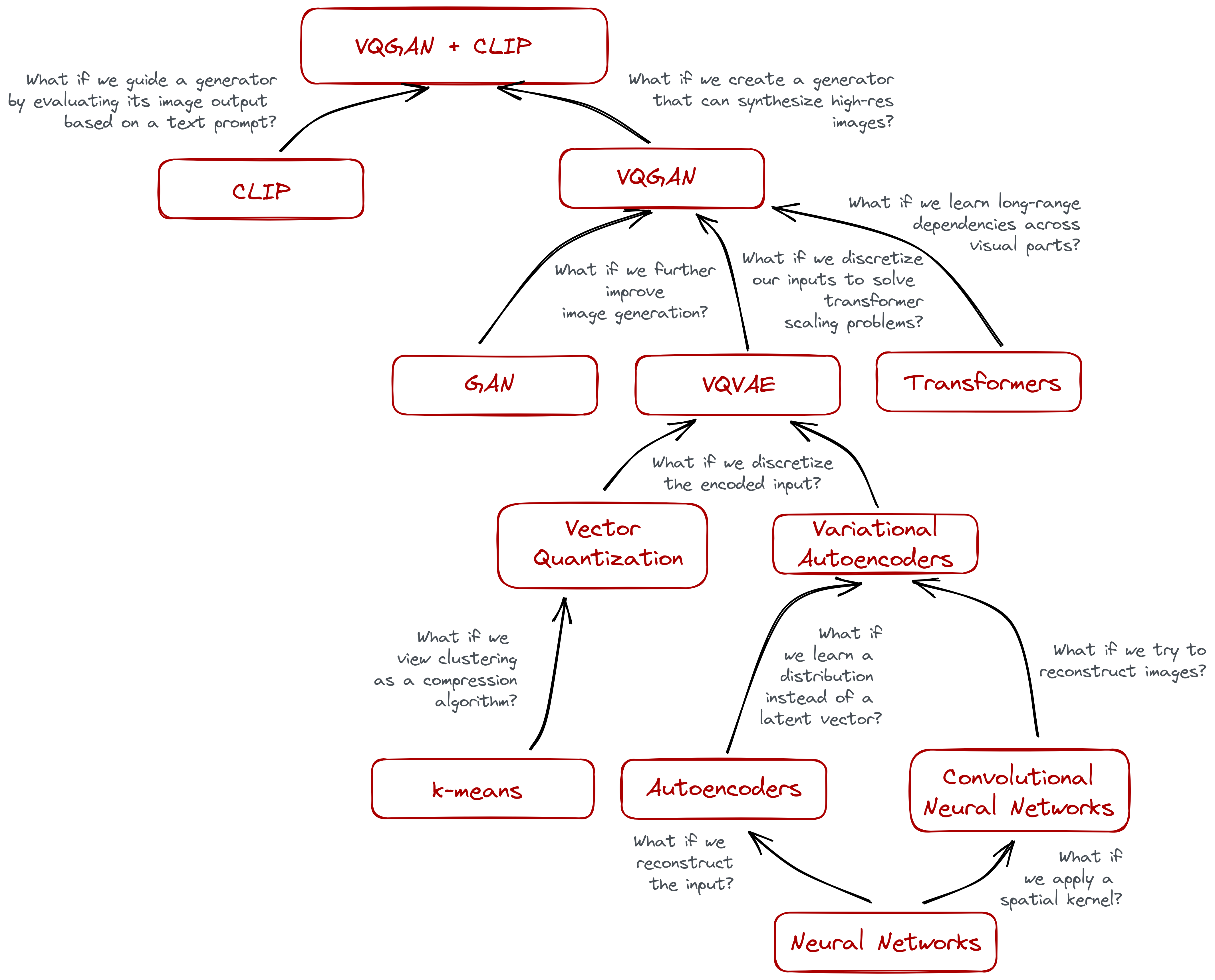
This may be helpful for someone who aren’t familiar yet with other intermediate architectures like autoencoders and what-not. And may also be helpful as a study guide or concept map. I decided not to break down some concepts like CLIP and Transformers because a lot of resources are already available to understand them.
Again, this is opinionated and it reflects how I understood the building blocks of VQGAN. Of course, there’s a lot of work that preempts each idea, but I only wrote the ones that I find important. Let me know if I misrepresented anything by commenting below!
References
- Ballard, D.H., 1999. An introduction to natural computation. MIT press.
- Chen, M., Radford, A., Child, R., Wu, J., Jun, H., Luan, D. and Sutskever, I., 2020, November. Generative pretraining from pixels. In International Conference on Machine Learning (pp. 1691-1703). PMLR.
- Child, R., Gray, S., Radford, A. and Sutskever, I., 2019. Generating long sequences with sparse transformers. arXiv preprint arXiv:1904.10509.
- Dosovitskiy, A., Beyer, L., Kolesnikov, A., Weissenborn, D., Zhai, X., Unterthiner, T., Dehghani, M., Minderer, M., Heigold, G., Gelly, S. and Uszkoreit, J., 2020. An image is worth 16x16 words: Transformers for image recognition at scale. arXiv preprint arXiv:2010.11929.
- Esser, P., Rombach, R. and Ommer, B., 2021. Taming transformers for high-resolution image synthesis. In Proceedings of the IEEE/CVF Conference on Computer Vision and Pattern Recognition (pp. 12873-12883).
- Goodfellow, I., Pouget-Abadie, J., Mirza, M., Xu, B., Warde-Farley, D., Ozair, S., Courville, A. and Bengio, Y., 2020. Generative adversarial networks. Communications of the ACM, 63(11), pp.139-144.
- Gu, J., Wang, Z., Kuen, J., Ma, L., Shahroudy, A., Shuai, B., Liu, T., Wang, X., Wang, G., Cai, J. and Chen, T., 2018. Recent advances in convolutional neural networks. Pattern Recognition, 77, pp.354-377.
- Isola, P., Zhu, J.Y., Zhou, T. and Efros, A.A., 2017. Image-to-image translation with conditional adversarial networks. In Proceedings of the IEEE conference on computer vision and pattern recognition (pp. 1125-1134).
- Johnson, J., Alahi, A. and Fei-Fei, L., 2016, October. Perceptual losses for real-time style transfer and super-resolution. In European conference on computer vision (pp. 694-711). Springer, Cham.
- Mnih, A. and Gregor, K., 2014, June. Neural variational inference and learning in belief networks. In International Conference on Machine Learning (pp. 1791-1799). PMLR.
- Oord, A.V.D., Vinyals, O. and Kavukcuoglu, K., 2017. Neural discrete representation learning. arXiv preprint arXiv:1711.00937.
- Parmar, N., Vaswani, A., Uszkoreit, J., Kaiser, L., Shazeer, N., Ku, A. and Tran, D., 2018, July. Image transformer. In International Conference on Machine Learning (pp. 4055-4064). PMLR.
- Radford, A., Kim, J.W., Hallacy, C., Ramesh, A., Goh, G., Agarwal, S., Sastry, G., Askell, A., Mishkin, P., Clark, J. and Krueger, G., 2021. Learning transferable visual models from natural language supervision. arXiv preprint arXiv:2103.00020.
- Salakhutdinov, R. and Hinton, G., 2009, April. Deep boltzmann machines. In Artificial intelligence and statistics (pp. 448-455). PMLR.
- Weissenborn, D., Täckström, O. and Uszkoreit, J., 2019. Scaling autoregressive video models. arXiv preprint arXiv:1906.02634.
- Vaswani, A., Shazeer, N., Parmar, N., Uszkoreit, J., Jones, L., Gomez, A.N., Kaiser, Ł. and Polosukhin, I., 2017. Attention is all you need. In Advances in neural information processing systems (pp. 5998-6008).
Changelog
- 08-12-2021: Replace the Lenna example with a picture of a cat.
- 08-09-2021: Update title from “Taming transformers” to “The Illustrated” as suggested by a friend.
-
You might see VQGAN-CLIP being written as CLIP-VQGAN, CLIP+VQGAN, or VQGAN+CLIP. The order doesn’t matter and the dash symbol isn’t an operation. They’re all the same thing. ↩
-
It may not be how we perceive the world around us, but it may be how we sense it. Note that our eyes are composed of cone cells that respond differently to different wavelengths. We can treat these cones analogous to a pixel’s RGB channels. ↩
-
I will admit that this analogy may be a stretch. However, I’d like to think that even if we reason in a symbolic manner, the way information travels to us is through a continuous variation of light wavelengths. As they say, analogies work until they don’t. I may be stretching it a bit far in this column. ↩
-
I labeled the pixel-based approach as continuous to complete the story. When normalized, you can think of pixel values as a number between 0 to 1, each representing the intensity or presence of that color. ↩
-
Again, treat this paragraph with a grain of salt. It’s difficult to truly interpret (i.e., rigorously and empirically) what each codeword represents, moreso their interactions once fed to a transformer. For explanation’s sake, just know that at the end of the vector quantization process, we now have discrete inputs that can easily scale with our transformer network. ↩