Implementing a two-layer neural network from scratch

I am currently following the course notes of CS231n: Convolutional Neural Networks for Visual Recognition in Stanford University. There are programming exercises involved, and I wanted to share my solutions to some of the problems.

In this exercise, a two-layer fully-connected artificial neural network (ANN) was developed in order to perform classification in the CIFAR-10 dataset. The full-implementation is done through the following steps:

• Toy model creation
• ANN Implementation
  • Architecture set-up
  • Forward Pass: Loss computation
  • Backward Pass: Gradient Computation
  • Batch Training
  • Prediction
• Toy model testing
• Training
• Hyperparameter Tuning
• Results

Toy Model Creation

It is first important to build a small neural network in order to test our loss and gradient computations. This can then save us time and effort when debugging our code. Here, we will create a toy model, and a toy dataset in order to check our implementations:

input_size = 4
hidden_size = 10
num_classes = 3
num_inputs = 5

def init_toy_model():
  np.random.seed(0)
  return TwoLayerNet(input_size, hidden_size, num_classes, std=1e-1)

def init_toy_data():
  np.random.seed(1)
  X = 10 * np.random.randn(num_inputs, input_size)
  y = np.array([0, 1, 2, 2, 1])
  return X, y

net = init_toy_model()
X, y = init_toy_data()

Remember that np.random.seed was used so that our experiments are repeatable. This function makes the random numbers predictable. Thus, if we have a seed reset, the same numbers will appear every time. Again, the reason we do this is because we are implementing code that uses random numbers (i.e., np.random.randn) and if we want to debug this, we need this random number generator to output the same numbers in the meantime. The answer of John1024 in StackOverflow is also a good explanation of this function.

Artificial Neural Network (ANN) Implementation

In this section, we will implement the forward and backward passes of the ANN, and then write code for batch training and prediction. But first, let us examine the architecture of the neural net.

Architecture set-up

The neural network architecture can be seen below:

Figure 1: Articificial Neural Network Architecture

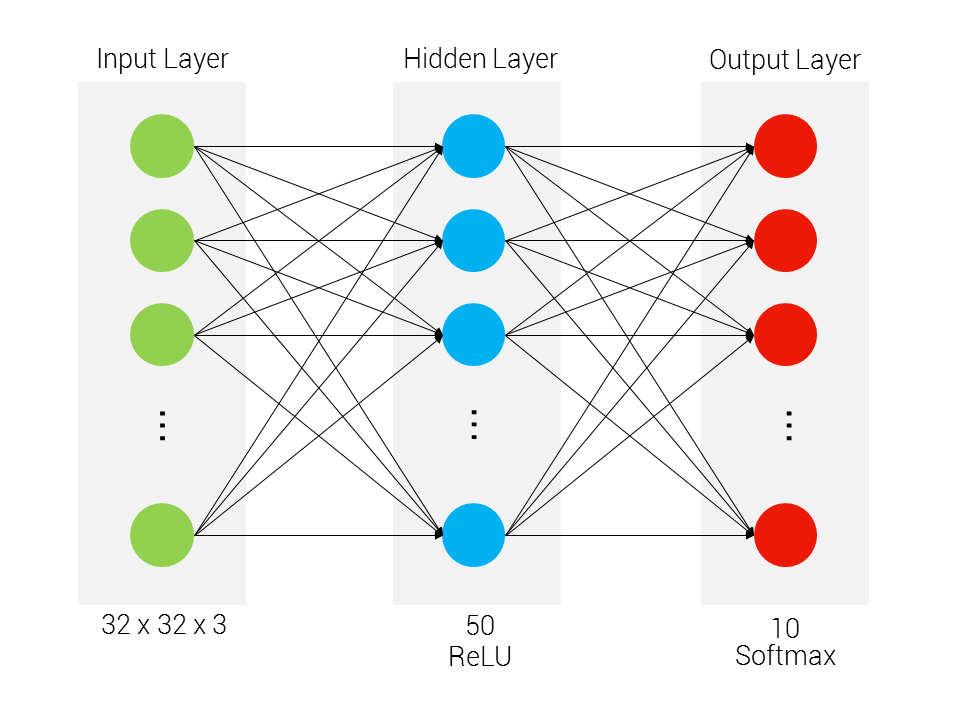
There are two layers in our neural network (note that the counting index starts with the first hidden layer up to the output layer). Moreover, the topology between each layer is fully-connected. For the hidden layer, we have ReLU nonlinearity, whereas for the output layer, we have a Softmax loss function.

The “vertical size” of the neural network for the input and output layers is dependent on the CIFAR-10 input and classes respectively, while the hidden layer is arbitrarily set.

Thus, given an input dimension of D, a hidden layer dimension of H, and number of classes C, we have the following weight and bias shapes:

W1: First layer weights; has shape (D, H)
b1: First layer biases; has shape (H,)
W2: Second layer weights; has shape (H, C)
b2: Second layer biases; has shape (C,)

Forward Pass: Loss computation

Before we compute the loss, we need to first perform a forward pass. Because we are implementing a fully-connected layer, the forward pass is simply a straightforward dot matrix operation. We then compute for the pre-activation values z1 and z2 for the hidden and output layers respectively, and the activation for the first layer.

# First layer pre-activation
z1 = X.dot(W1) + b1

# First layer activation
a1 = np.maximum(0, z1)

# Second layer pre-activation
z2 = a1.dot(W2) + b2

scores = z2

The scores variable keeps the pre-activation values for the output layer. We will be using this in a while to find the activation values in the output layer, and consequently the cross-entropy loss.

So for the second-layer activation, we have:

# Second layer activation
exp_scores = np.exp(scores)
a2 = exp_scores / np.sum(exp_scores, axis=1, keepdims=True)

And to compute for the loss, we perform the following code:

corect_logprobs = -np.log(a2[range(N), y])
data_loss = np.sum(corect_logprobs) / N
reg_loss = 0.5 * reg * np.sum(W1 * W1) + 0.5 * reg * np.sum(W2 * W2)
loss = data_loss + reg_loss

Backward Pass: Gradient Computation

We now implement the backward pass, where we compute the derivatives of the weights and biases and propagate them across the network. In this way, the network gets a feel of the contributions of each individual units, and adjusts itself accordingly so that the weights and biases are optimal.

We first compute for the gradients, thus we have:

dscores = a2
dscores[range(N),y] -= 1
dscores /= N

And then we propagate them back to our network:

# W2 and b2
grads['W2'] = np.dot(a1.T, dscores)
grads['b2'] = np.sum(dscores, axis=0)

# Propagate to hidden layer
dhidden = np.dot(dscores, W2.T)

# Backprop the ReLU non-linearity
dhidden[a1 <= 0] = 0

# Finally into W,b
grads['W1'] = np.dot(X.T, dhidden)
grads['b1'] = np.sum(dhidden, axis=0)

We should not also forget to regularize our gradients:

grads['W2'] += reg * W2
grads['W1'] += reg * W1

Batch Training

In our TwoLayerNet class, we also implement a train() function that trains the neural network using stochastic gradient descent. First, we create a random minibatch of training data and labels, then we store them in X_batch and Y_batch respectively:

sample_indices = np.random.choice(np.arange(num_train), batch_size)
X_batch = X[sample_indices]
y_batch = y[sample_indices]

And then we update our parameters in our network.

self.params['W1'] += -learning_rate * grads['W1']
self.params['b1'] += -learning_rate * grads['b1']
self.params['W2'] += -learning_rate * grads['W2']
self.params['b2'] += -learning_rate * grads['b2']

Prediction

Lastly, we implement a predict() function that classifies our inputs with respect to the scores and activations found after the output layer. We simply make a forward pass for the input, and then get the maximum of the scores that was found.

z1 = X.dot(self.params['W1']) + self.params['b1']
a1 = np.maximum(0, z1) # pass through ReLU activation function
scores = a1.dot(self.params['W2']) + self.params['b2']
y_pred = np.argmax(scores, axis=1)

Toy model testing

Once we’ve implemented our functions, we can then test them to see if they are working properly. The IPython notebook tests our implementation by checking our computed scores with respect to the correct scores hardcoded in the program.

In the first test, we got a difference of 3.68027206479e-08

Your scores:
[[-0.81233741 -1.27654624 -0.70335995]
 [-0.17129677 -1.18803311 -0.47310444]
 [-0.51590475 -1.01354314 -0.8504215 ]
 [-0.15419291 -0.48629638 -0.52901952]
 [-0.00618733 -0.12435261 -0.15226949]]

correct scores:
[[-0.81233741 -1.27654624 -0.70335995]
 [-0.17129677 -1.18803311 -0.47310444]
 [-0.51590475 -1.01354314 -0.8504215 ]
 [-0.15419291 -0.48629638 -0.52901952]
 [-0.00618733 -0.12435261 -0.15226949]]

For the second and third tests, we check the difference between the loss and the correct loss, as well as the relative error between our backward passes:

Difference between your loss and correct loss:
1.79856129989e-13


b2 max relative error: 4.447635e-11
W1 max relative error: 3.561318e-09
W2 max relative error: 3.440708e-09
b1 max relative error: 2.738421e-09

We then test our neural network’s training ability by checking if our loss is decreasing. What we will do is to plot our loss history, and verify that it is actually decreasing.

Figure 2: Plot of loss history on toy dataset

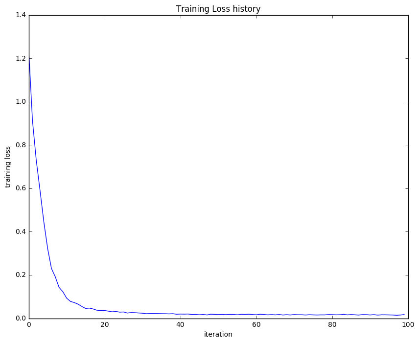
It seems like our loss is decreasing and our errors are relatively low. This suggests that our functions are working well and our forward and backward pass implementations are on point. Because we’re already confident with our code, we can then start training our neural network in the real dataset. I will not show how the data was loaded and preprocessed because it simply follows a similar structure as with previous exercises. So we will dive straight to training instead.

Training

We first train our neural network with the following parameters (as given in the exercise):

stats = net.train(X_train, y_train, X_val, y_val,
            num_iters=1000, batch_size=200,
            learning_rate=1e-4, learning_rate_decay=0.95,
            reg=0.5, verbose=True)

Given these parameters, we achieve a validation accuracy of 0.287, and it is not particularly good. Remember that our k-Nearest Neighbor classifier can actually perform relatively the same. In fact, if we plot our loss history and classification accuracy history, we see some troubling signs:

Figure 3: Plot of loss and classification accuracy on CIFAR-10

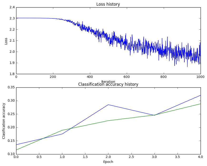
As of now, we can see that our loss function is decreasing in a non-linear fashion. It looks weird and it may suggest a low learning rate. Moreover, we can also see that there is no gap between the training and validation model, and this may suggest that our model has very low capacity.

We can also visualize the weights of our network, in this case, we arrive at the following:

Figure 4: Visualization of ANN Weights using default parameters

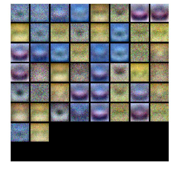
We can see from here that the network is learning a set of weights that are very similar to one another. One can see a lot of car classes in this network. Because of this “homogeneity,” any input is often misclassified by the network.

What we will be doing next is to tune our hyperparameters, and try to achieve a good score.

Hyperparameter Tuning

We then tune our parameters by sweeping through different values of learning rates and regularization strengths. For this implementation, I would like to attribute MyHumbleSelf’s solution as my basis for finding a good combination of parameters.

best_val = -1
best_stats = None
learning_rates = [1e-2, 1e-3]
regularization_strengths = [0.4, 0.5, 0.6]
results = {}
iters = 2000
for lr in learning_rates:
    for rs in regularization_strengths:
        net = TwoLayerNet(input_size, hidden_size, num_classes)

        # Train the network
        stats = net.train(X_train, y_train, X_val, y_val,
                    num_iters=iters, batch_size=200,
                    learning_rate=lr, learning_rate_decay=0.95,
                    reg=rs)

        y_train_pred = net.predict(X_train)
        acc_train = np.mean(y_train == y_train_pred)
        y_val_pred = net.predict(X_val)
        acc_val = np.mean(y_val == y_val_pred)

        results[(lr, rs)] = (acc_train, acc_val)

        if best_val < acc_val:
            best_stats = stats
            best_val = acc_val
            best_net = net

# Print out results.
for lr, reg in sorted(results):
    train_accuracy, val_accuracy = results[(lr, reg)]
    print('lr %e reg %e train accuracy: %f val accuracy: %f' % (
                lr, reg, train_accuracy, val_accuracy))

print('best validation accuracy achieved during cross-validation: %f' % best_val)

From here, we were able to ramp up our validation accuracy up to 0.497000. This is particularly good compared to our SVM and Softmax Implementation. If we visualize the learned weights, we can obtain the following figure:

Figure 5: Visualization of ANN Weights after tuning

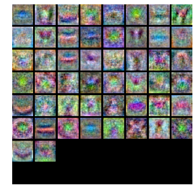
We can then see that the weights are more heterogeneous. This can then accommodate more classes for a given set of inputs. Personally, what I like about this is that it looks like an acid trip.

Results

Lastly, we implement our learned weights into our network, and check the test accuracy. For my implementation, I got 0.496