Implementing a multiclass support-vector machine
I am currently following the course notes of CS231n: Convolutional Neural Networks for Visual Recognition in Stanford University. There are programming exercises involved, and I wanted to share my solutions to some of the problems.
In this notebook, a Multiclass Support Vector Machine (SVM) will be implemented. For this exercise, a linear SVM will be used.
Linear classifiers differ from k-NN in a sense that instead of memorizing the whole training data every run, the classifier creates a “hypothesis” (called a parameter), and adjusts it accordingly during training time. This “adjustment” is then achieved through an optimization algorithm, in this case, via Stochastic Gradient Descent (SGD). The full implementation will be done through the following steps:
- Data Loading and Preprocessing
- SVM classifier Implementation
- Stochastic Gradient Descent
- Hyperparameter Tuning
- Results
Data Loading and Preprocessing
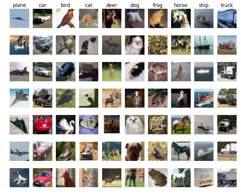
Similar with the other exercise, the CIFAR-10 dataset is also being utilized. As a simple way of sanity-checking, we load and visualize a subset of this training example as shown below:
Splitting and reshaping the data
Here, we split the data into training, validation, and test sets. Moreover, a small development set will be created from our training data. Moreover, we also reshape the image data into different rows. We can then arrive with the following sizes for our data:
Training data shape:  (49000, 3072)
Validation data shape:  (1000, 3072)
Test data shape:  (1000, 3072)
dev data shape:  (500, 3072)
Computing and subtracting the mean image
In machine learning, it is standard procedure to normalize the input features (or pixels, in the case of images) in such a way that the data is centered and the mean is removed. For images, a mean image is computed across all training images and then subtracted from our datasets.
In Python, we can easily compute for the mean image by using np.mean. In
this regard, we have:
# Compute for the mean image
mean_image = np.mean(X_train, axis=0)
print(mean_image[:10]) # print a few of the elements

# Visualize the mean image
plt.figure(figsize=(4,4))
plt.imshow(mean_image.reshape((32,32,3)).astype('uint8'))
plt.show()
Visualizing the mean image leads us to this figure
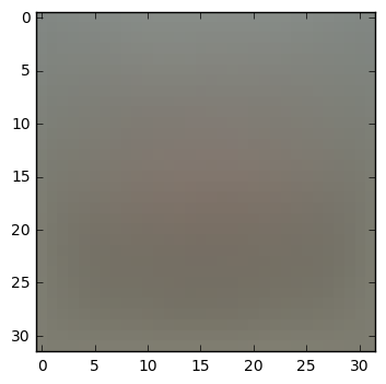
We then subtract this mean image from our training and test data. Furthermore, we also append our bias matrix (made up of ones) so that our optimizer will treat both the weights and biases at the same time.
# Subtract the mean image from train and test data
X_train -= mean_image
X_val -= mean_image
X_test -= mean_image
X_dev -= mean_image

# Append the bias dimension of ones (i.e. bias trick) so that our SVM
# only has to worry about optimizing a single weight matrix W.
X_train = np.hstack([X_train, np.ones((X_train.shape[0], 1))])
X_val = np.hstack([X_val, np.ones((X_val.shape[0], 1))])
X_test = np.hstack([X_test, np.ones((X_test.shape[0], 1))])
X_dev = np.hstack([X_dev, np.ones((X_dev.shape[0], 1))])

print(X_train.shape, X_val.shape, X_test.shape, X_dev.shape)
This gives an additional dimension to our datasets:
(49000, 3073) (1000, 3073) (1000, 3073) (500, 3073)
SVM Classifier Implementation
The set-up behind the Multiclass SVM Loss is that for a query image, the SVM prefers that its correct class will have a score higher than the incorrect classes by some margin \(\Delta\).
In this case, for the pixels of image \(x_{i}\) with label \(y_{i}\), we compute for the score for each class \(j\) as \(s_{j} \equiv f(x_{i}, W)\). We then describe the behavior stated above in the following equation:
\[L_{i} = \sum_{j \neq y_{i}} max(0,s_{j} - s_{y_{i}} + \Delta)\]For our purposes, we will often deal with the equation shown above. A
thorough discussion of SVM can (obviously) be found in the course
notes. We will then build the
SVM classifier found in linear_svm.py by first filling-in the gradient
computation, and then implementing its vectorized version.
Gradient Computation
In order to implement the code for the gradient, we simply go back to the representation of our loss function in SVM. In fact, we can can represent the equation above as the following:
\[L_{i} = \sum_{j \neq y_{i}} max(0,w_{j}^{T}x_{i} - w_{y_{i}}^{T}x_{i} + \Delta)\]In order to obtain the gradient, we need to differentiate this function with respect to \(w_{y_{i}}\) and \(w_{j}\):
\[\nabla_{w_{y_{i}}} L_{i} = - \left(\sum_{j \neq y_{i}} 1 (w_{j}^{T}x_{i} - w_{y_{i}}^{T}x_{i} + \Delta > 0)\right)x_{i}\] \[\nabla_{w_{j}} L_{i} = 1 (w_{j}^{T}x_{i} - w_{y_{i}}^{T}x_{i} + \Delta > 0) x_{i}\]For the equation above, we only count the number of classes that didn’t pass through the margin (\(j \neq y_{i}\)). Remember that sometimes, a given example’s class will not always be classified correctly (or given a higher score). The SVM loss function then penalizes these mishaps. So for every example, we sum all the incorrect classes that was computed, and \(x_{i}\) is scaled by that number.
In Python, we can implement a naive computation for the the gradient by this code:
# Compute for the loss and gradient
num_classes = W.shape[1]
num_train = X.shape[0]
loss = 0.0

for i in range(num_train):
  # For each training example, we will count the
  # scores and keep track of the correct class score
  scores = X[i].dot(W)
  correct_class_score = scores[y[i]]

  for j in range(num_classes):
  # We then compare it for each class
      if j == y[i]:
          continue

      # Compute the margin
      margin = scores[j] - correct_class_score + 1

      # If margin is greater than zero, the class
      # contributes to the loss. And the gradient
      # is computed
      if margin > 0:
          loss += margin
          dW[:,y[i]] -= X[i,:]
          dW[:,j] += X[i,:]
This means that for each data example, we compute the scores, and take note of the score of the correct class.
Then we compare the scores for each class . We then compute for the margin
and see if it is greater than 0. Take note that certain data examples can
be classified incorrectly (i.e., a ship, because of its blue-ish background,
may be mistaken as an airplane in a blue sky). This then contributes to our
loss.
For the gradient, we simply count the number of classes that didn’t meet the
margin, and this will contribute to our gradient vector dW. The expression
dW[:,y[i]] -= X[i,:] is analogous to \(\nabla_{w_{y_{i}}} L_{i}\) as
dW[:,j] += X[i,:] is to \(\nabla_{w_{j} L_{i}}\).
Also, don’t forget to sum the gradient over all training examples and regularize it.
# Divide all over training examples
dW /= num_train
# Add regularization
dW += reg * W
Vectorized implementation of loss and gradient computation
Implementing a vectorized computation for the loss is quite simple. First we
compute the scores of the input with respect to the weights, and then we keep
track of the scores, and get the maximum (with respect to 0) as it is being
stored to the variable margin. Most of these are achievable using the
numpy library:
num_train = X.shape[0]
delta = 1.0

# Compute for the scores
scores = X.dot(W)

# Record the score of the example's correct class
correct_class_score = scores[np.arange(num_train), y]

# Compute for the margin by getting the max between 0 and the computed expression
margins = np.maximum(0, scores - correct_class_score[:,np.newaxis] + delta)
margins[np.arange(num_train), y] = 0

# Add all the losses together
loss = np.sum(margins)

# Divide the loss all over the number of training examples
loss /= num_train

# Regularize
loss += 0.5 * reg * np.sum(W * W)
In order to implement the vectorized version of our gradient computation, we first create a mask that flags the examples when their margin is greater than 0., and then, we proceed normally by counting the number of these examples:
# This mask can flag the examples in which their margin is greater than 0
X_mask = np.zeros(margins.shape)
X_mask[margins > 0] = 1

# As usual, we count the number of these examples where margin > 0
count = np.sum(X_mask,axis=1)
X_mask[np.arange(num_train),y] = -count

dW = X.T.dot(X_mask)

# Divide the gradient all over the number of training examples
dW /= num_train

# Regularize
dW += reg*W
Stochastic Gradient Descent
Remember that our main objective is to minimize the loss that was computed by our SVM. One way to do that is through gradient descent. Given then gradient vector that we have obtained earlier, we simply “move” our parameters to the direction that our gradient is pointing.
self.W += -learning_rate * grad
We can then train our SVM classifier using gradient descent and plot the loss with respect to the number of iterations.
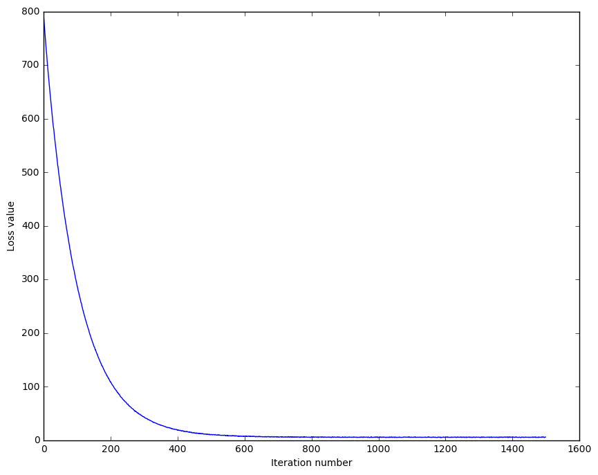
We see that the curve is smooth (due to regularization), and is descending. We can then infer that our SVM and cost implementations are correct. Normally, fuzzy curves are caused by non-regularized losses. It may be an important point of experiment later on.
If we use the trained parameters to predict our classes, we often arrive at the following results:
training accuracy: 0.363959
validation accuracy: 0.382000
We can still improve our accuracies by tuning our learning rate and regularization hyperparameters.
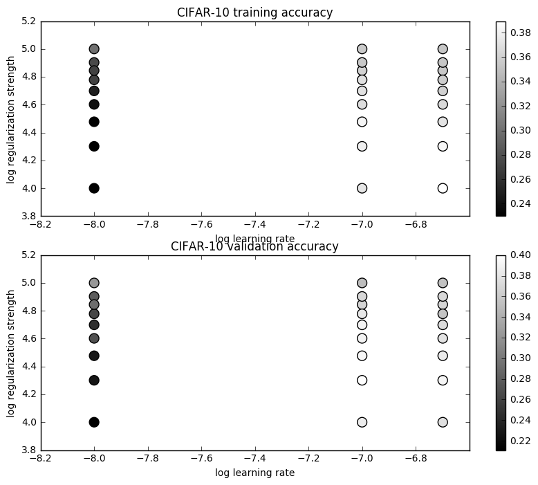
Hyperparameter Tuning
One good way to tune our hyperparameters is to train and test our classifier over a matrix of values. In this case, we are training our SVM classifier with a matrix containing learning rate and regularization values. We then record their accuracies, and take the maximum value we encounter. Normally, the set of parameters that obtained the maximum accuracy can be deemed as a good hyperparameter setting.
For my implementation, I would like to give credit to bruceoutdoors’ for providing a good set of working values for the learning rate and regularization strengths.
learning_rates = [1e-8, 1e-7, 2e-7]
regularization_strengths = [1e4, 2e4, 3e4, 4e4, 5e4, 6e4, 7e4, 8e4, 1e5]
We can then visualize our values so that we can observe the behavior of our hyperparameters:
Results
Using the best set of hyperparameters that we have, we can then visualize the learned weights for each class. These weights can serve as “templates” for our classifier when comparing to a test example.
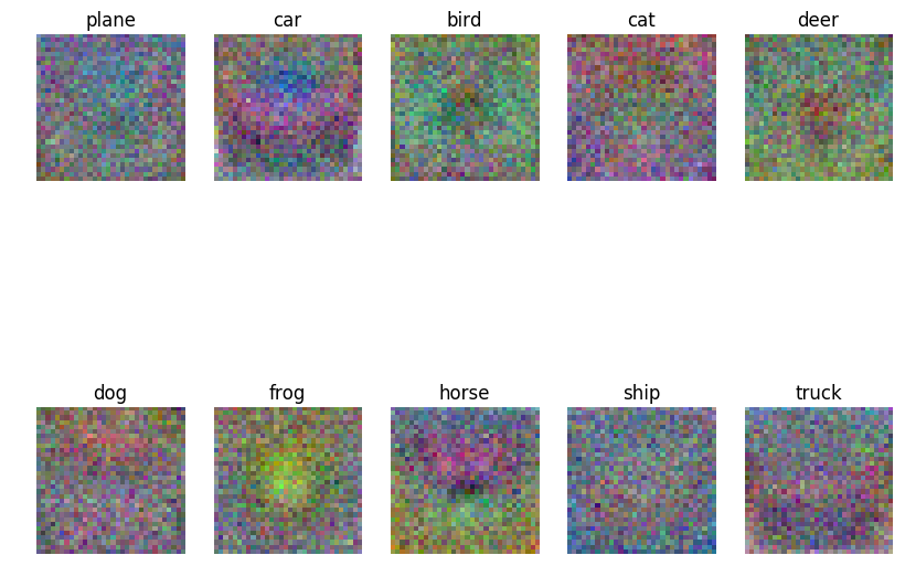
Above, we can see how some classes, such as the ship and plane class,
have pretty similar templates. This can be attributed to the fact that the
background of both vehicles are blue, and this can often lead to
misclassification. In order to test our parameters, we predict again using
our SVM classifier, and we can obtain the following result:
linear SVM on raw pixels final test set accuracy: 0.380000
Here we can see an improvement from our k-NN classifier, both in terms of accuracy and speed. By using a linear classifier, we eliminate the need to memorize the training data and look into it every time we see a test example. Instead, what we do is that we create a hypothesis of the training set, build a template, and compare these test examples into the template that we have built.