Implementing a k-Nearest Neighbor classifier

I am currently following the course notes of CS231n: Convolutional Neural Networks for Visual Recognition in Stanford University. There are programming exercises involved, and I wanted to share my solutions to some of the problems.

The basic idea for the k-Nearest Neighbors classifier is that we find the k closest images in the dataset with respect to our query x. Here, we will perform the following processes:

• Load the CIFAR-10 dataset
• Compute for the L2 (Euclidean) Distance
  • Two-Loop Implementation
  • One-Loop Implementation
  • No-Loop Implementation
• Visualize the distances
• Perform cross-validation to find the best k

Load the CIFAR-10 Dataset

CIFAR-10 is a labeled dataset that houses 80 million tiny images. It was created by Alex Krizhevsky, Vinod Nair, and Geoffrey Hinton. It contains 60,000 32x32 color images with 6,000 images per class.

We can visualize some examples in CIFAR-10, here we can see a sample of 10 classes with 7 examples each.

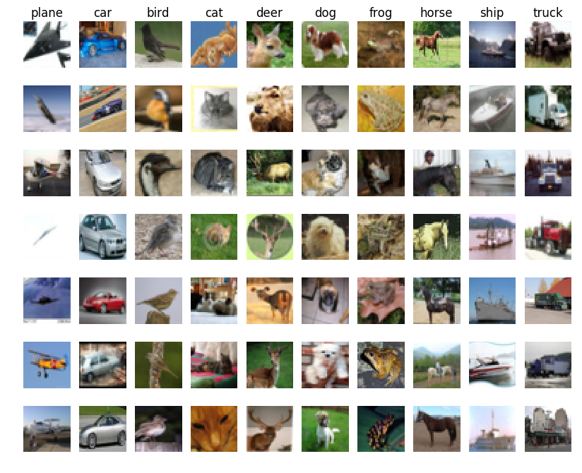
Figure 1: Samples of the CIFAR-10 Dataset

As we can see, for each class, there are distinct images related to it. For example, the car class is represented by different car images, some of which have different orientation or color. These images then make-up a certain “template” that can be used by the classifier in order to categorize a test image.

Compute for the L2 Distance

Distance computation is a quantifiable means of comparing two images together. To compute for distance, pixel-wise differences are often implemented. In this method, distance is computed “pixel-by-pixel” and then the elements of the corresponding matrix is added together. Highly similar images will have lower values while different images will have higher values. Moreover, images that are exactly similar have a 0 distance. The choice of distance that was used in the assignment is the L2 distance:

\[d_{2}(I_{1}, I_{2}) = \sqrt{\sum_{p}(I_{1}^{p} - I_{2}^{p})^{2}}\]

Thus, for images \(I_{1}\) and \(I_{2}\), we perform a sum of squares pixel computation for each \(p\) and then get the square root. The assignment requires us to implement the L2 distance in three different ways.

Two-loop implementation

The two-loop computation uses a nested-loop in order to compute for the pixel-wise L2 Distance between the test and train images. This is one of the easiest methods to implement, but it takes a toll on speed because of the looping nature.

num_test = X.shape[0]
num_train = self.X_train.shape[0]
dists = np.zeros((num_test, num_train))
for i in xrange(num_test):
  for j in xrange(num_train):
    dists[i,j] = np.linalg.norm(self.X_train[j,:]-X[i,:])
return dists

Here, I am implementing the np.linalg.norm function to compute for the norm (which is, in a sense, equivalent to the L2 equation) of X_train and X. Furthermore, this can also be implemented by religiously following the equation above, and thus we can have something similar below:

dists[i,j] = np.sqrt(np.sum(np.square(X[i,:]-self.X_train[j,:])))

One-loop implementation

For the one-loop implementation, what we do is that in our dists matrix, we compute for the distances for each example in the test set X against the examples in the training set X_train. As we will see, instead of filling the dists matrix cell-by-cell (as we have done in the two-loop computation), we fill the dists matrix row-by-row, or in other words, by “test example by test example.”

num_test = X.shape[0]
num_train = self.X_train.shape[0]
dists = np.zeros((num_test, num_train))
for i in xrange(num_test):
  dists[i, :] = np.linalg.norm(self.X_train - X[i,:], axis = 1)

This is intuitively faster than the previous implementation, because the distance computation against the training set is done in parallel. In the next implementation, we will implement a fully-vectorized computation that can further improve the speed of our computations.

No-loop implementation

The no-loop computation is a fully-vectorized implementation of the L2 distance. This eliminates the loops entirely, replacing a cell by cell (or row by row) implementation into a single matrix solution.

My workaround for this is to implement another form of the L2 Distance, which can actually be derived from the equation above. In this case, for two vectors \(\mathbf{I}_{1}\) and \(\mathbf{I}_{2}\). We can also compute for the L2 Distance as:

\[d_{2}(\mathbf{I}_{1}, \mathbf{I}_{2}) = \left\lvert \left\lvert \mathbf{I}_{1} - \mathbf{I}_{2} \right\rvert \right\rvert = \sqrt{\left\lvert \left\lvert\mathbf{I}_{1} \right\rvert \right\rvert^{2} + \left\lvert \left\lvert \mathbf{I}_{2}\right\rvert \right\rvert^{2} - 2 \mathbf{I}_{1} \cdot \mathbf{I}_{2}}\]

With this equation, we can easily compute for the dists matrix without using any loops, for this we implement the following:

num_test = X.shape[0]
num_train = self.X_train.shape[0]
dists = np.zeros((num_test, num_train))
dists = np.sqrt((X**2).sum(axis=1)[:, np.newaxis] + (self.X_train**2).sum(axis=1) - 2 * X.dot(self.X_train.T))

The vectorized version can in fact provide a very fast performance compared to the looped implementations. Using my own machine, I was able to obtain the following execution times:

Two loop version took 92.134323 seconds
One loop version took 213.639710 seconds
No loop version took 6.479004 seconds

We were then able to reduce the time it takes to compute for the L2 Distance in a large dataset from 3 minutes to just 6 seconds. Very impressive indeed!

You may notice that the one-loop implementation is much slower than the two-loop implementation, and it goes against the intuition that we had. The course instructors mentioned that the problem is system dependent and it’s nothing to worry about. Source: badmephisto’s answer in “Assignment#1 knn -single loop slower than double loop”

Visualize the distances

We can plot the dists matrix and visualize the distances of our test examples with respect to different training examples. Here, as you look down, we are looking at a representation of our test examples. As you look from left to right, we see the training examples. Thus we have over 500 test examples and over 5000 training examples. Darker regions represent areas of low distance (more similar images) while lighter regions represent areas of high distance (more different images).

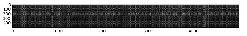
Figure 2: Visualization of the dists matrix

The distinctly visible rows (say, the dark rows in the 300 mark or the white rows in the 400 mark) represent test examples that are similar (or different) to most of the training examples. Let’s focus on the dark rows in the 300 mark. The reason why distinct dark rows can be seen in it is because there could be many classes in the training set that was found to be similar to it. This can be attributed to similar backgrounds or hues that can confuse our classifier into thinking that it belongs to the same class.

On the other hand, the columns we see are in fact training examples that are not similar to any of the test examples. Perhaps a certain training example was found to have no any significant similarity to any of the test examples. This will then result to a high L2 distance, and consequently, generate a white column into our visualization.

Perform cross-validation to find the best k

One good method to know the best value of k, or the best number of neighbors that will do the “majority vote” to identify the class is through cross-validation. What we will do here is to split the training set into 5 folds, and compute the accuracies with respect to an array of k choices. From this we sort the accuracies and obtain the best value of k.

Firt we split the training set X_train:

num_folds = 5
k_choices = [1, 3, 5, 8, 10, 12, 15, 20, 50, 100]

X_train_folds = []
y_train_folds = []

X_train_folds = np.array_split(X_train, num_folds)
y_train_folds = np.array_split(y_train, num_folds)

And then we perform cross-validation. Thus, for each k value, we will run the k-NN algorithm num_folds times. Here we will use all but one folds as our training data, and the last one as our validation set. We then store the accuracies of each fold and all values of k in the k_to_accuracies dictionary.

for k in k_choices:
    k_to_accuracies[k] = []

for k in k_choices:
    print('k=%d' % k)
    for j in range(num_folds):
        # Use all but one folds as our crossval training set
        X_train_crossval = np.vstack(X_train_folds[0:j] + X_train_folds[j+1:])
        # Use the last fold as our crossval test set
        X_test_crossval = X_train_folds[j]

        y_train_crossval = np.hstack(y_train_folds[0:j]+y_train_folds[j+1:])
        y_test_crossval = y_train_folds[j]

        # Train the k-NN Classifier using the crossval training set
        classifier.train(X_train_crossval, y_train_crossval)

        # Use the trained classifer to compute the distance of our crossval test set
        dists_crossval = classifier.compute_distances_no_loops(X_test_crossval)

        y_test_pred = classifier.predict_labels(dists_crossval, k)
        num_correct = np.sum(y_test_pred == y_test_crossval)
        accuracy = float(num_correct) / num_test

        k_to_accuracies[k].append(accuracy)

In order to see how the value of k changes with respect to our cross validation set, we can visualize them in terms of line plot with error bars:

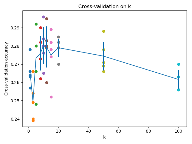
Figure 3: Visualization of the cross-validation procedure with different k values

From now, we can choose a good k value. Let’s take k = 10.

Got 141 / 500 correct => accuracy: 0.282000

And thus we were able to obtain an accuracy of 28.2%. It is not as good as state-of-the-art classifiers today (a Convolutional Neural Network solution in Kaggle was able to reach a whopping 95%). But this is a good start to learn the image classification pipeline and the efficiency of the vectorization method.

Changelog

• 12-16-2018: Update cross-validation plot, thanks @earnshae for spotting the error!