Solving the Inverse Kinematics problem using Particle Swarm Optimization

In this notebook, I solved a 6-DOF Inverse Kinematics problem by treating it as an optimization problem. In this case, I implemented Particle Swarm Optimization (PSO) in order to find an optimal solution from a set of candidate solutions.

Introduction

Inverse Kinematics (IK) is one of the most challenging problems in robotics. The problem involves finding an optimal pose for a manipulator given the position of the end-tip effector. This can be seen in contrast with forward kinematics, where the end-tip position is sought given the pose or joint configuration. Normally, this position is expressed as a point in a coordinate system (e.g., in a Cartesian system, it is a point comprising of \(x\), \(y\), and \(z\) coordinates.). On the other hand, the manipulator’s pose can be expressed as the collection of joint variables that can describe the angle of bending or twist (in revolute joints) or length of extension (in prismatic joints).

IK is particularly difficult because multiple solutions can arise. Intuitively, a robotic arm can have multiple ways of reaching through a certain point. Moreover, calculation can prove to be very difficult. Simple solutions can be found for 3-DOF manipulators, but a 6-DOF or higher can be very challenging to solve algebraically.

IK Problem as an Optimization Problem

In this implementation, I am using the same set-up during my forward kinematics project as shown here. I am using a 6-DOF Stanford Manipulator, with 5 revolute joints and 1 prismatic joint. Furthermore, my constraints are similar as before, and it’s shown in the table below:

Parameters	Lower Boundary	Upper Boundary
\(\theta_1\)	\(-\pi\)	\(\pi\)
\(\theta_2\)	\(-\frac{\pi}{2}\)	\(\frac{\pi}{2}\)
\(d_3\)	\(1\)	\(3\)
\(\theta_4\)	\(-\pi\)	\(\pi\)
\(\theta_5\)	\(-\frac{5\pi}{36}\)	\(\frac{5\pi}{36}\)
\(\theta_6\)	\(-\pi\)	\(\pi\)

Table 1: Joint variable physical constraints

Now, if we’re given with an end-tip position (in this case, an \(xyz\) coordinate), we need to find the optimal parameters with the constraints imposed above. These conditions are then sufficient in order to treat this problem as an optimization problem. We should then define our parameters \(\mathbf{X}\) as:

\[\mathbf{X} \equiv \begin{bmatrix} \theta_{1} & \theta_{2} & d_{3} & \theta_{5} & \theta_{6} \end{bmatrix}\]

And then we impose the end-tip position as a target \(\mathbf{T}\) as:

\[\mathbf{T} \equiv \begin{bmatrix} T_{x} & T_{y} & T_{z} \end{bmatrix}\]

We can then start implementing our optimization algorithm.

Initializing the Swarm

The main idea for PSO is that we set a swarm \(\mathbf{S}\) composed of particles \(\mathbf{P}_{n}\) into a search space in order to find the optimal solution. The movement of the swarm depends on the cognitive (\(c_{1}\)) and social (\(c_{2}\)) behavior of the particles composing it. The cognitive component speaks of the particle’s bias towards its personal best from its past experience (i.e., how attracted is it to its own best position). The social component controls how the particles are attracted to the best score found by the swarm (or global best). High \(c_{1}\) and low \(c_{2}\) can often cause the swarm to stagnate. The inverse can cause the swarm to converge very fast, resulting to suboptimal solutions. A visualization of its effect can be found here.

We then define our particle \(\mathbf{P}\) as:

\[\mathbf{P} \equiv \mathbf{X} = \begin{bmatrix} \theta_{1} & \theta_{2} & d_{3} & \theta_{5} & \theta_{6} \end{bmatrix}\]

And define the swarm as being composed of particles \(\mathbf{P}_{n}\) with certain positions at a timestep t:

\[\mathbf{S}_{t} \equiv \begin{bmatrix} \mathbf{P}_{1} & \mathbf{P}_{2} & \mathbf{P}_{3} & \ldots & \mathbf{P}_{N} \end{bmatrix}\]

In my implementation, I designated \(\mathbf{P}_{1}\) as the initial configuration of the manipulator at zero-position. This means that the angles are at 0 degrees and the link offset is also zero. I then generated the other \(N-1\) particles using a uniform distribution where it is controlled by the hyperparameter \(\epsilon\).

currentPos = np.random.uniform(0,1,epsilon, size_params]) * options[4] + params.T

Finding the global best solution

In order to find the global best solution, the swarm must then be moved. This movement is then translated by an update of the current position given the swarm velocity \(V\). That is,

\[\mathbf{S}_{t+1} = \mathbf{S}_{t} + \mathbf{V}_{t+1}\]

The velocity is then computed as the following:

\[\mathbf{V}_{t+1} = w\mathbf{V}_{t} + c_{1}r_{t}[y_{ij} - x_{ij}] + c_{2}r_{2}[y - x_{ij}]\]

Where \(y_{ij}\) and \(y_{j}\) are the personal and global best scores, respectively. Moreover, \(w\) is the inertia weight that controls the “memory” of the swarm’s previous position. In Python, this can be written as:

# Update velocity
cognitive = (options[1] * np.random.uniform(0,1,[1,6])) * (pBestPos[particle,:] - currentPos[particle,:])
social = (options[2] * np.random.uniform(0,1,[1,6])) * (gBestPos - currentPos[particle,:])
velocityMatrix[particle,:] = (options[3] * velocityMatrix[particle,:]) + cognitive + social

# Update position
currentPos[particle,:] = currentPos[particle,:] + velocityMatrix[particle,:]

Simulation Results

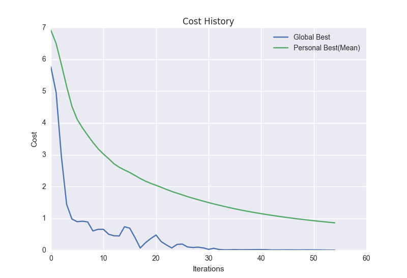
I tested my inverse kinematics implementation by letting the particles find an optimal joint configuration for the point (-2,2,3). My PSO parameters are the following: c_1 = c_2 = 1.5, swarmSize = 20, w = 0.5, and epsilon = 1.0. I plotted the particle movement (in terms of their end-tip positions) in a 3D coordinate system, and made it into a GIF. Moreover, the proceeding chart shows the cost history of a single run.

Figure 1: Inverse Kinematics Simulation

Figure 2: Cost History

Execution Time

The average execution time (in 10 trials) for my simulation is: 1.099 seconds.

I also ran a test to see the performance speed of PSO. For 10 trials, I generated a random point \((x,y,z)\) and fed it into the algorithm. I then computed for the mean and I got 0.8971 seconds.

Conclusion

This simple experiment showed that a 6-DOF inverse kinematics problem can be solved by treating it as an optimization problem. A standard PSO global best algorithm with inertia weights was implemented and the results showed that it can achieve the desired end-tip position in almost a second. The choice of the optimization algorithm is purely personal, I enjoy implementing PSO and it’s one of my go-to algorithms when testing out things. This notebook is a simple proof-of-concept that an algebraically difficult problem can be solved in a different way. Other optimization algorithms can be used, and it may even reduce the execution time so that IK problems can be solved in almost real-time.

Access the gist here.

Table of Contents: