Solving the Forward Kinematics of a Stanford Arm
This is my implementation of the forward kinematics problem in Robotics. The forward kinematics problem involves finding the end-tip position of a manipulator in a coordinate space given its joint parameters (i.e., joint angles for revolute joints and link offset for prismatic joints). This means that given a certain pose of a robotic arm, the xyz coordinates of the hand must be determined. For this implementation, I will be using the 6-DOF Stanford Manipulator as my basis.
Stanford Arm
The Stanford Arm, designed by Victor Scheinmann in 1969, can be considered to be one of the classic manipulators in robotics, and is one of the first robots that are designed exclusively for computer control. In this project, I performed a forward kinematics procedure in simulating the arm.
Forward Kinematics uses different kinematic equations in order to compute for the end-tip position of a manipulator given its joint parameters. Joint parameters can refer to joint angles \(\theta\) for revolute joints, or link lengths for prismatic joints. In solving for the Forward Kinematics, I utilized the Denavit-Hartenberg (DH) Parameters.
Methodology
Denavit Hartenberg Parameters
With DH Parameters, solving for the Forward Kinematics is easy. I only need to take four parameters for each joint \(i\): \(\theta_{i}\) for the joint angle, \(\alpha_{i}\) for the link twist, \(d_{i}\) for the link offset, and \(a_{i}\) for the link length. Once I’ve obtained them, I can just plug them in to this transformation matrix:
\[T_{i-1}^{i} = \begin{bmatrix} \cos(\theta_{i}) & -cos(\alpha_{i})\cdot sin(\theta_{i}) & \sin(\alpha_{i})\cdot\sin(\theta_{i}) & a_{i} \cdot cos(\theta_{i}) \\ \sin(\theta_{i}) & cos(\alpha_{i}) \cdot cos(\theta_{i}) & -sin(\alpha_{i}) \cdot cos(\theta_{i}) & a_{i} \cdot sin(\theta_{i}) \\ 0 & sin(\alpha_{i}) & cos(\alpha_{i}) & d_{i} \\ 0 & 0 & 0 & 1 \end{bmatrix}\]For the Stanford Arm, here are the DH Parameters:
| Joint | Joint Angle | Link Offset | Link Length | Link Twist |
|---|---|---|---|---|
| 1 | \(\theta_{1}\) | \(d_{1}\) | 0 | -90 |
| 2 | \(\theta_{2}\) | \(d_{2}\) | 0 | -90 |
| 3 | -90 | \(d_{3}\) | 0 | 0 |
| 4 | \(\theta_{4}\) | \(d_{4}\) | 0 | -90 |
| 5 | \(\theta_{5}\) | 0 | 0 | 90 |
| 6 | \(\theta_{6}\) | \(d_{6}\) | 0 | 0 |
The joint variables are then expressed as a vector \(V\):
\[V \equiv \begin{bmatrix} \theta_{1} & \theta_{2} & d_{3} & \theta_{5} & \theta_{6} \end{bmatrix}\]They are then limited in terms of physical constraints, such that:
| Parameters | Limitation |
|---|---|
| \(\theta_1\) | [-180 180] |
| \(\theta_2\) | [-90 90] |
| \(d_3\) | [1 3] |
| \(\theta_4\) | [-180 180] |
| \(\theta_5\) | [-25 25] |
| \(\theta_6\) | [-180 180] |
MATLAB Implementation
The following code snippets will show my implementation of the forward kinematics of the Stanford Manipulator in MATLAB.
Transformation Matrix
The transformation matrix is expressed as the function getTransformMatrix.
It takes the DH parameters of a single joint as its input argument, and
outputs the corresponding transformation matrix \(T_{i-1}^{i}\).
function [T] = getTransformMatrix(theta, d, a, alpha)
T = [cosd(theta) -sind(theta) * cosd(alpha) sind(theta) * sind(alpha) a * cosd(theta);...
     sind(theta) cosd(theta) * cosd(alpha)  -cosd(theta) * sind(alpha) a * sind(theta);...
     0,sind(alpha),cosd(alpha),d;...
     0,0,0,1];
end
Forward Kinematics
Forward kinematics then becomes a simple implementation of the
getTransformMatrix above. By setting the link lengths constant, the end-tip
position can be computed. In my case, I wrapped this function inside the
method forwardKinematics:
function [T00,T01,T12,T23,T34,T45,T56,Etip] =  forwardKinematics(theta1,theta2,d3,theta4,theta5,theta6)

T00 = [1 0 0 0; 0 1 0 0; 0 0 1 0; 0 0 0 1];
T01 = getTransformMatrix(theta1,d1,0,-90);
T12 = getTransformMatrix(theta2,d2,0,90);
T23 = getTransformMatrix(0,d3,0,-90);
T34 = getTransformMatrix(theta4,d4,0,-90);
T45 = getTransformMatrix(theta5,0,0,90);
T56 = getTransformMatrix(theta6,d6,0,0);

Etip = T00 * T01 * T12 * T23 * T34 * T45 * T56;

end
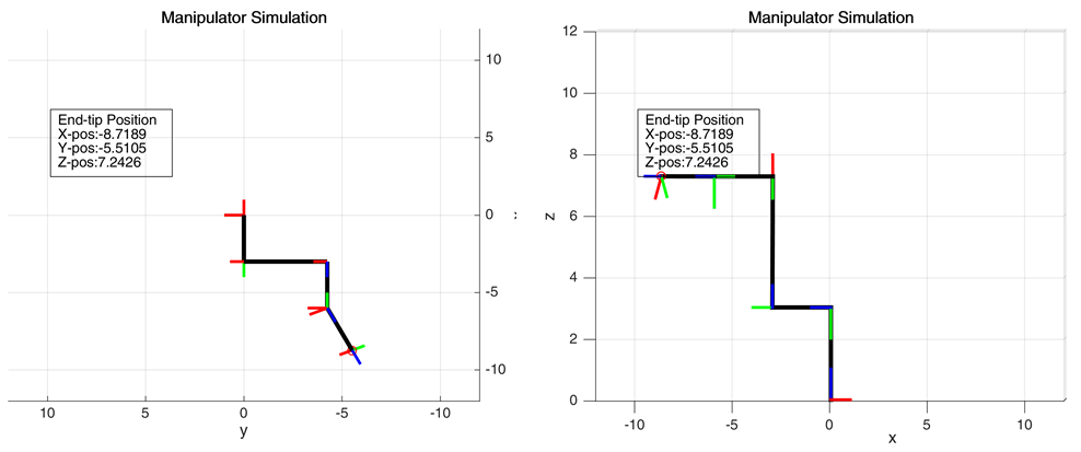
Simulation Results
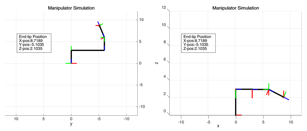
Here are some simulations of my work. I tried different values for the joint parameters and then recorded the results in GIF format. I also plotted the top and side views just to see how the manipulator is posed in terms of the x-y and x-z coordinates.
Simulation 1
\(\theta_{1}\) = -90, \(\theta_{2}\) = 90, \(d_{3}\) = 6, \(\theta_{4}\) = 45, \(\theta_{5}\) = 25, \(\theta_{6}\) = 90

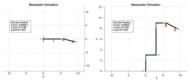
Simulation 2
\(\theta_{1}\) = 180, \(\theta_{2}\) = 0, \(d_{3}\) = 6, \(\theta_{4}\) = 45, \(\theta_{5}\) = 25, \(\theta_{6}\) = 0
Simulation 3
\(\theta_{1}\) = 90, \(\theta_{2}\) = -45, \(d_{3}\) = 6, \(\theta_{4}\) = 45, \(\theta_{5}\) = -25, \(\theta_{6}\) = 45

Conclusion
Solving for the end-tip position given the joint parameters (or doing forward kinematics) is much easier algebraically when one is using the DH parameters. It is then a lot easier to model a manipulator because four parameters are only needed in order to define a certain joint.
Limitations should also be imposed in the model with respect to the physical environment it belongs to. This is to avoid “impractical” or “illogical” movements being done by the manipulator.
Solving for the inverse kinematics proved to be very difficult algebraically. Multiple solutions often arise and it must always be checked with respect to the physical constraints imposed.